Midterm 2 Solutions: Difference between revisions
JoseKolbLugo (talk | contribs) (New page: Image:MOSFET pic.png) |
(→d)) |
||
| (31 intermediate revisions by 2 users not shown) | |||
| Line 1: | Line 1: | ||
==Problem 1== | |||
'''Consider a magnetic system described by an Ising model <math>(S_i = \pm1)</math> on a square lattice with <math>\ H = \sum_{\langle ij\rangle} J_{ij} s_i s_{j} + \sum_{\langle ij\rangle} K_{ij} s_i s_{j} </math>. Here, the ferromagnetic interaction <math> \ J_{ij} < 0 </math> couples only nearest-neighbor spins. In contrast,the antiferromagnetic interaction <math>\ K_{ij}>0 </math> couples only the the second neighbors, i.e. spins that are "across the square" ( diagonally placed relative to each other). Here, the ferromagnetic interaction <math>\ J_{ij} < 0</math> couples only the nearest-neighbor spins. In contrast, the anti ferromagnetic interaction <math>\ K_{ij} > 0 </math> couples only the second neighbors, i.e. spins that are "across the square" (diagonally placed relative to each other. ''' | |||
===a)=== | |||
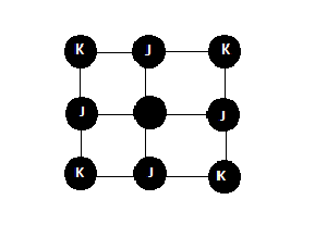
'''Sketch the suare lattice and determine the number of first neighbors <math>\Z_{FM}</math> which interact ferromagnetically with the given spin, and the number of second neighbors <math>\Z_{AFM}</math> which interact antiferromagnetically with the given spin. (5points)''' | |||
[[Image:lattice.png]] | |||
Image of square lattice with ferromagnetic <math>J_{i,j} <0</math> coupling nearest neighbor spins. | |||
Anti-ferromagnetic <math>K_{i,j} <0</math> coupling only second nearest neighbors. | |||
<math>Z_{FM} =4</math> | |||
<math>Z_{AFM} =4</math> | |||
===b)=== | |||
'''Use the mean-field approximation, where <math>\ S_{i} S_{j} \rightarrow S_{i} \langle S_{j} \rangle</math>. Assume that the magnitude of <math>\ J_{ij}</math> is appreciably larger then the magnitude of <math>\ K_{ij}</math>; then the system will order ferromagnetically at low temperatures, so that <math>\langle S_{i} \rangle = m </math> for any site. Derive the self consistency condition determining the magnetization "m". (15points)''' | |||
The point of the mean-field approximation is to simplify a many body problem. To consider all the interactions taking place in a material would require huge amounts of computing power and resources. The mean-field approximation accomplishes this by considering only the average of the interactions. | |||
The first step in this problem is to right down our equation for the energy when <math> \ J_{ij}</math> is "appreciably larger than <math> \ K_{ij}</math> . | |||
<math>\ H = \sum_{ij} J_{ij} S_{i} S_{j}</math> | |||
We also know: | |||
<math>\langle S_{i} \rangle = m </math> | |||
This is due to the fact that we are considering many neighbors, so as z gets very large then we get the following: | |||
<math>\ 1/z \sum_{j=1}^z S_{j} \rightarrow \langle S_{i} \rangle = m </math> | |||
Now if we sum over many random variables we get the following: | |||
<math> \sum_{j=1}^z S_j \rightarrow z\langle S_{i} \rangle</math> | |||
Now we can simplify our original expression as the following: | |||
<math>\ H = J \sum_{i}^N S_{i} zm</math> | |||
Pulling out the constants we get: | |||
<math>\ H = Jzm \sum_{i=1}^N S_{i} </math> | |||
Since we have a problem of non interacting spins in an internal field we can consider and solve for only one spin. This then gives us the following: | |||
<math>\ H = JzmS_{1}</math> | |||
<math>\ S_{1} = \pm 1</math> | |||
Now we need to consider the probability for the spin to point either up or down. This is given as the following: | |||
<math>\ P( S_{1} = \pm 1) = 1/z (e^{ \pm Jzm/kt}) </math> | |||
We can also define z as: | |||
<math> \ z = e^{ \pm Jzm/kt}</math> | |||
Now we can define the magnetization as the spin times the probability of the spin: | |||
<math>\ m = \sum_{S_{1} = \pm 1} S_{1} P(S_{1})</math> | |||
Rewriting this equation we get: | |||
<math> \ m = \frac {e^{ Jzm/kt} - e^{ -Jzm/kt} }{e^{Jzm/kt} + e^{ -Jzm/kt}} </math> | |||
This is the same as the tanh, so we get: | |||
<math> \ m = \tanh( \frac{Jzm}{kt})</math> | |||
Making <math>\ \beta = 1/kt</math> | |||
We get: | |||
<math>\ m = \tanh ( \beta Jzm)</math> | |||
===c)=== | |||
'''Determine the Curie Temperature <math>\ T_{c}</math>. (10 points)''' | |||
<math>\ T_{c} = Jz</math> | |||
===d)=== | |||
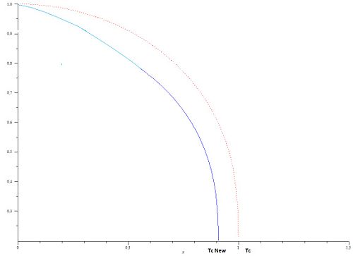
'''Now imagine that we increase the strength of the anti ferromagnetic coupling <math>\ K_{ij}</math> between the second neighbors. Sketch how <math>\ T_{c}</math> changes, and find the condition giving <math>\ T_{c} \rightarrow 0 </math>. The phenomenon that the ordering temperature can be reduced due to "competing" interactions is called "magnetic frustration".(10 points)''' | |||
[[Image:changeTc.jpg|center|500px]] | |||
===e)=== | |||
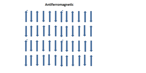
'''Now imagine that <math>\ J_{ij} </math> is very small (in magnitude). so that the anti ferromagnetic interactions between the second neighbors dominate. Sketch the ground state configuration of the spins in this case. Determine the (Neel) temperature <math>\ T_{N}</math> where the magnetic order is lost, assuming that <math>\ J_{ij} = 0</math> but <math>\ K_{ij}</math> remains finite. (10 points)''' | |||
[[Image:antiferromagnetic.png|center|thumb|500px]] | |||
===f)=== | |||
'''EXTRA CREDIT QUESTION: Plot the phase diagram of this model, as a function of <math>\ K/J</math> and <math>\ T</math>, indicating the phases and phase transitions.(20 points)''' | |||
==Problem 2== | |||
'''Consider a system of electrons moving in two dimensions.''' | |||
===a)=== | |||
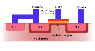
'''Give some example, and sketch a device where this can be experimentally realized. Where do we find applications of such devices?(5 points)''' | |||
[[Image:MOSFET pic.png]] | [[Image:MOSFET pic.png]] | ||
===b)=== | |||
'''Electrons interact through electrostatic Coulomb interactions, but there exists a density regime where the interactions can be ignored. Does this happen at low density or at high density? Give a physical argument supporting your statement. (5 points)''' | |||
Since Coulomb interactions are long range by <math>e^2/r</math> high densities cause the formation of solids such as crystals. | |||
===c)=== | |||
'''Now assume that we work in the regime where the interactions can be ignored, so that we can approximate the electrons as a gas of free particles obeying Fermi Dirac statistics(Pauli exclusion principle). The solutions of the Schroedinger equation for free particles are plain waves with wave- vector <math> \vec{k}</math>. Assuming that this system of electrons is contained in a finite area container of side L, use periodic boundary conditions to determine the allowed values for the wave-vector.(10 points)''' | |||
When we put any wave into a cavity such as a guitar the allowed wave vectors become quantized. We also know that the Schroedinger equation <math> \ E(k) = \frac{\hbar^{2} k^{2}}{2m}</math> has discrete allowed values which leads to energy levels. Th allowed values of the wave-vector then become: | |||
<math> \Delta k = \frac{2 \pi}{L}</math> | |||
===d)=== | |||
'''Determine the Fermi energy of this system as a function of the density of electrons n.(10 points)''' | |||
We can start from the definition of the number of electrons. This can be shown as the sum over all k values, times the probability that the states are occupied, and times the number of states. | |||
<math>\ N = 2 \sum_{\left\vert \vec{k} \right\vert < k_{f}} f( \epsilon_{k})</math> | |||
Because we are assuming we are at zero temperature, our values are sharply defined. With this information, and when we have k vector less than k fermi, we can then make our probability equal to one giving us: | |||
<math>\ N = 2 \sum_{\left\vert \vec{k} \right\vert < k_{f}} 1 </math> | |||
When summing over all k we need to sum over the individual components. | |||
<math>\ N = 2 \sum_{kx} \sum_{ky} 1 </math> | |||
Changing our summation into an integral we get: | |||
<math>\ N = 2A \int\limits_{0}^{k_{f}} \frac{d^{2}k}{(2 \pi )^2}</math> | |||
Now changing to polar coordinates we get: | |||
<math>\ N = 2A \int\limits_{0}^{k_{f}} \frac{2 \pi k dk}{(2 \pi )^2} </math> | |||
Now we can simplify our expression: | |||
<math>\ N = \frac{ 4 \pi A}{(2 \pi )^2}\int\limits_{0}^{k_{f}} k dk</math> | |||
<math>\ \frac{N}{A} = \frac{4 \pi k^2}{8 \pi^2}</math> | |||
Using the fact that <math>\ \frac{N}{A} = n </math> we get: | |||
<math>\ n = \frac{k^2}{2 \pi}</math> | |||
<math>\ k^2 = n 2 \pi</math> | |||
Plugging this into <math>\ E(k) = \frac{\hbar^2 k^2}{2m}</math>: | |||
<math>\ E_{f} = \frac{\hbar n 2 \pi}{2m}</math> | |||
So our fermi energy then becomes: | |||
<math>\ E_{f} = \frac{\hbar n \pi}{m}</math> | |||
===e)=== | |||
'''Determine the average kinetic energy of(all) the electrons in the ground state, as a function of n.(15 points)''' | |||
===f)=== | |||
'''What is the temperature range where Fermi-Dirac statistics and all quantum effects can be ignored?(5 points)''' | |||
Where <math>T \rightarrow \infty</math> Fermi-Dirac Statistics and all quantum effects can be ignored. | |||
Latest revision as of 21:42, 11 April 2011
Problem 1
Consider a magnetic system described by an Ising model Failed to parse (SVG (MathML can be enabled via browser plugin): Invalid response ("Math extension cannot connect to Restbase.") from server "https://wikimedia.org/api/rest_v1/":): {\displaystyle (S_i = \pm1)} on a square lattice with Failed to parse (SVG (MathML can be enabled via browser plugin): Invalid response ("Math extension cannot connect to Restbase.") from server "https://wikimedia.org/api/rest_v1/":): {\displaystyle \ H = \sum_{\langle ij\rangle} J_{ij} s_i s_{j} + \sum_{\langle ij\rangle} K_{ij} s_i s_{j} } . Here, the ferromagnetic interaction Failed to parse (SVG (MathML can be enabled via browser plugin): Invalid response ("Math extension cannot connect to Restbase.") from server "https://wikimedia.org/api/rest_v1/":): {\displaystyle \ J_{ij} < 0 } couples only nearest-neighbor spins. In contrast,the antiferromagnetic interaction Failed to parse (SVG (MathML can be enabled via browser plugin): Invalid response ("Math extension cannot connect to Restbase.") from server "https://wikimedia.org/api/rest_v1/":): {\displaystyle \ K_{ij}>0 } couples only the the second neighbors, i.e. spins that are "across the square" ( diagonally placed relative to each other). Here, the ferromagnetic interaction Failed to parse (SVG (MathML can be enabled via browser plugin): Invalid response ("Math extension cannot connect to Restbase.") from server "https://wikimedia.org/api/rest_v1/":): {\displaystyle \ J_{ij} < 0} couples only the nearest-neighbor spins. In contrast, the anti ferromagnetic interaction Failed to parse (SVG (MathML can be enabled via browser plugin): Invalid response ("Math extension cannot connect to Restbase.") from server "https://wikimedia.org/api/rest_v1/":): {\displaystyle \ K_{ij} > 0 } couples only the second neighbors, i.e. spins that are "across the square" (diagonally placed relative to each other.
a)
Sketch the suare lattice and determine the number of first neighbors Failed to parse (SVG (MathML can be enabled via browser plugin): Invalid response ("Math extension cannot connect to Restbase.") from server "https://wikimedia.org/api/rest_v1/":): {\displaystyle \Z_{FM}} which interact ferromagnetically with the given spin, and the number of second neighbors Failed to parse (SVG (MathML can be enabled via browser plugin): Invalid response ("Math extension cannot connect to Restbase.") from server "https://wikimedia.org/api/rest_v1/":): {\displaystyle \Z_{AFM}} which interact antiferromagnetically with the given spin. (5points)
Image of square lattice with ferromagnetic Failed to parse (SVG (MathML can be enabled via browser plugin): Invalid response ("Math extension cannot connect to Restbase.") from server "https://wikimedia.org/api/rest_v1/":): {\displaystyle J_{i,j} <0}
 coupling nearest neighbor spins.
Anti-ferromagnetic Failed to parse (SVG (MathML can be enabled via browser plugin): Invalid response ("Math extension cannot connect to Restbase.") from server "https://wikimedia.org/api/rest_v1/":): {\displaystyle K_{i,j} <0}
 coupling only second nearest neighbors.
Failed to parse (SVG (MathML can be enabled via browser plugin): Invalid response ("Math extension cannot connect to Restbase.") from server "https://wikimedia.org/api/rest_v1/":): {\displaystyle Z_{FM} =4}

Failed to parse (SVG (MathML can be enabled via browser plugin): Invalid response ("Math extension cannot connect to Restbase.") from server "https://wikimedia.org/api/rest_v1/":): {\displaystyle Z_{AFM} =4}
b)
Use the mean-field approximation, where Failed to parse (SVG (MathML can be enabled via browser plugin): Invalid response ("Math extension cannot connect to Restbase.") from server "https://wikimedia.org/api/rest_v1/":): {\displaystyle \ S_{i} S_{j} \rightarrow S_{i} \langle S_{j} \rangle} . Assume that the magnitude of Failed to parse (SVG (MathML can be enabled via browser plugin): Invalid response ("Math extension cannot connect to Restbase.") from server "https://wikimedia.org/api/rest_v1/":): {\displaystyle \ J_{ij}} is appreciably larger then the magnitude of Failed to parse (SVG (MathML can be enabled via browser plugin): Invalid response ("Math extension cannot connect to Restbase.") from server "https://wikimedia.org/api/rest_v1/":): {\displaystyle \ K_{ij}} ; then the system will order ferromagnetically at low temperatures, so that Failed to parse (SVG (MathML can be enabled via browser plugin): Invalid response ("Math extension cannot connect to Restbase.") from server "https://wikimedia.org/api/rest_v1/":): {\displaystyle \langle S_{i} \rangle = m } for any site. Derive the self consistency condition determining the magnetization "m". (15points)
The point of the mean-field approximation is to simplify a many body problem. To consider all the interactions taking place in a material would require huge amounts of computing power and resources. The mean-field approximation accomplishes this by considering only the average of the interactions.
The first step in this problem is to right down our equation for the energy when Failed to parse (SVG (MathML can be enabled via browser plugin): Invalid response ("Math extension cannot connect to Restbase.") from server "https://wikimedia.org/api/rest_v1/":): {\displaystyle \ J_{ij}} is "appreciably larger than Failed to parse (SVG (MathML can be enabled via browser plugin): Invalid response ("Math extension cannot connect to Restbase.") from server "https://wikimedia.org/api/rest_v1/":): {\displaystyle \ K_{ij}} .
Failed to parse (SVG (MathML can be enabled via browser plugin): Invalid response ("Math extension cannot connect to Restbase.") from server "https://wikimedia.org/api/rest_v1/":): {\displaystyle \ H = \sum_{ij} J_{ij} S_{i} S_{j}}
We also know:
Failed to parse (SVG (MathML can be enabled via browser plugin): Invalid response ("Math extension cannot connect to Restbase.") from server "https://wikimedia.org/api/rest_v1/":): {\displaystyle \langle S_{i} \rangle = m }
This is due to the fact that we are considering many neighbors, so as z gets very large then we get the following:
Failed to parse (SVG (MathML can be enabled via browser plugin): Invalid response ("Math extension cannot connect to Restbase.") from server "https://wikimedia.org/api/rest_v1/":): {\displaystyle \ 1/z \sum_{j=1}^z S_{j} \rightarrow \langle S_{i} \rangle = m }
Now if we sum over many random variables we get the following:
Failed to parse (SVG (MathML can be enabled via browser plugin): Invalid response ("Math extension cannot connect to Restbase.") from server "https://wikimedia.org/api/rest_v1/":): {\displaystyle \sum_{j=1}^z S_j \rightarrow z\langle S_{i} \rangle}
Now we can simplify our original expression as the following:
Failed to parse (SVG (MathML can be enabled via browser plugin): Invalid response ("Math extension cannot connect to Restbase.") from server "https://wikimedia.org/api/rest_v1/":): {\displaystyle \ H = J \sum_{i}^N S_{i} zm}
Pulling out the constants we get:
Failed to parse (SVG (MathML can be enabled via browser plugin): Invalid response ("Math extension cannot connect to Restbase.") from server "https://wikimedia.org/api/rest_v1/":): {\displaystyle \ H = Jzm \sum_{i=1}^N S_{i} }
Since we have a problem of non interacting spins in an internal field we can consider and solve for only one spin. This then gives us the following:
Failed to parse (SVG (MathML can be enabled via browser plugin): Invalid response ("Math extension cannot connect to Restbase.") from server "https://wikimedia.org/api/rest_v1/":): {\displaystyle \ H = JzmS_{1}}
Failed to parse (SVG (MathML can be enabled via browser plugin): Invalid response ("Math extension cannot connect to Restbase.") from server "https://wikimedia.org/api/rest_v1/":): {\displaystyle \ S_{1} = \pm 1}
Now we need to consider the probability for the spin to point either up or down. This is given as the following:
Failed to parse (SVG (MathML can be enabled via browser plugin): Invalid response ("Math extension cannot connect to Restbase.") from server "https://wikimedia.org/api/rest_v1/":): {\displaystyle \ P( S_{1} = \pm 1) = 1/z (e^{ \pm Jzm/kt}) }
We can also define z as:
Failed to parse (SVG (MathML can be enabled via browser plugin): Invalid response ("Math extension cannot connect to Restbase.") from server "https://wikimedia.org/api/rest_v1/":): {\displaystyle \ z = e^{ \pm Jzm/kt}}
Now we can define the magnetization as the spin times the probability of the spin:
Failed to parse (SVG (MathML can be enabled via browser plugin): Invalid response ("Math extension cannot connect to Restbase.") from server "https://wikimedia.org/api/rest_v1/":): {\displaystyle \ m = \sum_{S_{1} = \pm 1} S_{1} P(S_{1})}
Rewriting this equation we get:
Failed to parse (SVG (MathML can be enabled via browser plugin): Invalid response ("Math extension cannot connect to Restbase.") from server "https://wikimedia.org/api/rest_v1/":): {\displaystyle \ m = \frac {e^{ Jzm/kt} - e^{ -Jzm/kt} }{e^{Jzm/kt} + e^{ -Jzm/kt}} }
This is the same as the tanh, so we get:
Failed to parse (SVG (MathML can be enabled via browser plugin): Invalid response ("Math extension cannot connect to Restbase.") from server "https://wikimedia.org/api/rest_v1/":): {\displaystyle \ m = \tanh( \frac{Jzm}{kt})}
Making Failed to parse (SVG (MathML can be enabled via browser plugin): Invalid response ("Math extension cannot connect to Restbase.") from server "https://wikimedia.org/api/rest_v1/":): {\displaystyle \ \beta = 1/kt}
We get:
Failed to parse (SVG (MathML can be enabled via browser plugin): Invalid response ("Math extension cannot connect to Restbase.") from server "https://wikimedia.org/api/rest_v1/":): {\displaystyle \ m = \tanh ( \beta Jzm)}
c)
Determine the Curie Temperature Failed to parse (SVG (MathML can be enabled via browser plugin): Invalid response ("Math extension cannot connect to Restbase.") from server "https://wikimedia.org/api/rest_v1/":): {\displaystyle \ T_{c}} . (10 points)
Failed to parse (SVG (MathML can be enabled via browser plugin): Invalid response ("Math extension cannot connect to Restbase.") from server "https://wikimedia.org/api/rest_v1/":): {\displaystyle \ T_{c} = Jz}
d)
Now imagine that we increase the strength of the anti ferromagnetic coupling Failed to parse (SVG (MathML can be enabled via browser plugin): Invalid response ("Math extension cannot connect to Restbase.") from server "https://wikimedia.org/api/rest_v1/":): {\displaystyle \ K_{ij}} between the second neighbors. Sketch how Failed to parse (SVG (MathML can be enabled via browser plugin): Invalid response ("Math extension cannot connect to Restbase.") from server "https://wikimedia.org/api/rest_v1/":): {\displaystyle \ T_{c}} changes, and find the condition giving Failed to parse (SVG (MathML can be enabled via browser plugin): Invalid response ("Math extension cannot connect to Restbase.") from server "https://wikimedia.org/api/rest_v1/":): {\displaystyle \ T_{c} \rightarrow 0 } . The phenomenon that the ordering temperature can be reduced due to "competing" interactions is called "magnetic frustration".(10 points)
e)
Now imagine that Failed to parse (SVG (MathML can be enabled via browser plugin): Invalid response ("Math extension cannot connect to Restbase.") from server "https://wikimedia.org/api/rest_v1/":): {\displaystyle \ J_{ij} } is very small (in magnitude). so that the anti ferromagnetic interactions between the second neighbors dominate. Sketch the ground state configuration of the spins in this case. Determine the (Neel) temperature Failed to parse (SVG (MathML can be enabled via browser plugin): Invalid response ("Math extension cannot connect to Restbase.") from server "https://wikimedia.org/api/rest_v1/":): {\displaystyle \ T_{N}} where the magnetic order is lost, assuming that Failed to parse (SVG (MathML can be enabled via browser plugin): Invalid response ("Math extension cannot connect to Restbase.") from server "https://wikimedia.org/api/rest_v1/":): {\displaystyle \ J_{ij} = 0} but Failed to parse (SVG (MathML can be enabled via browser plugin): Invalid response ("Math extension cannot connect to Restbase.") from server "https://wikimedia.org/api/rest_v1/":): {\displaystyle \ K_{ij}} remains finite. (10 points)
f)
EXTRA CREDIT QUESTION: Plot the phase diagram of this model, as a function of Failed to parse (SVG (MathML can be enabled via browser plugin): Invalid response ("Math extension cannot connect to Restbase.") from server "https://wikimedia.org/api/rest_v1/":): {\displaystyle \ K/J} and Failed to parse (SVG (MathML can be enabled via browser plugin): Invalid response ("Math extension cannot connect to Restbase.") from server "https://wikimedia.org/api/rest_v1/":): {\displaystyle \ T} , indicating the phases and phase transitions.(20 points)
Problem 2
Consider a system of electrons moving in two dimensions.
a)
Give some example, and sketch a device where this can be experimentally realized. Where do we find applications of such devices?(5 points)
b)
Electrons interact through electrostatic Coulomb interactions, but there exists a density regime where the interactions can be ignored. Does this happen at low density or at high density? Give a physical argument supporting your statement. (5 points)
Since Coulomb interactions are long range by Failed to parse (SVG (MathML can be enabled via browser plugin): Invalid response ("Math extension cannot connect to Restbase.") from server "https://wikimedia.org/api/rest_v1/":): {\displaystyle e^2/r} high densities cause the formation of solids such as crystals.
c)
Now assume that we work in the regime where the interactions can be ignored, so that we can approximate the electrons as a gas of free particles obeying Fermi Dirac statistics(Pauli exclusion principle). The solutions of the Schroedinger equation for free particles are plain waves with wave- vector Failed to parse (SVG (MathML can be enabled via browser plugin): Invalid response ("Math extension cannot connect to Restbase.") from server "https://wikimedia.org/api/rest_v1/":): {\displaystyle \vec{k}} . Assuming that this system of electrons is contained in a finite area container of side L, use periodic boundary conditions to determine the allowed values for the wave-vector.(10 points)
When we put any wave into a cavity such as a guitar the allowed wave vectors become quantized. We also know that the Schroedinger equation Failed to parse (SVG (MathML can be enabled via browser plugin): Invalid response ("Math extension cannot connect to Restbase.") from server "https://wikimedia.org/api/rest_v1/":): {\displaystyle \ E(k) = \frac{\hbar^{2} k^{2}}{2m}} has discrete allowed values which leads to energy levels. Th allowed values of the wave-vector then become:
Failed to parse (SVG (MathML can be enabled via browser plugin): Invalid response ("Math extension cannot connect to Restbase.") from server "https://wikimedia.org/api/rest_v1/":): {\displaystyle \Delta k = \frac{2 \pi}{L}}
d)
Determine the Fermi energy of this system as a function of the density of electrons n.(10 points)
We can start from the definition of the number of electrons. This can be shown as the sum over all k values, times the probability that the states are occupied, and times the number of states.
Failed to parse (SVG (MathML can be enabled via browser plugin): Invalid response ("Math extension cannot connect to Restbase.") from server "https://wikimedia.org/api/rest_v1/":): {\displaystyle \ N = 2 \sum_{\left\vert \vec{k} \right\vert < k_{f}} f( \epsilon_{k})}
Because we are assuming we are at zero temperature, our values are sharply defined. With this information, and when we have k vector less than k fermi, we can then make our probability equal to one giving us:
Failed to parse (SVG (MathML can be enabled via browser plugin): Invalid response ("Math extension cannot connect to Restbase.") from server "https://wikimedia.org/api/rest_v1/":): {\displaystyle \ N = 2 \sum_{\left\vert \vec{k} \right\vert < k_{f}} 1 }
When summing over all k we need to sum over the individual components.
Changing our summation into an integral we get:
Now changing to polar coordinates we get:
Now we can simplify our expression:
Using the fact that we get:
Plugging this into :
So our fermi energy then becomes:
e)
Determine the average kinetic energy of(all) the electrons in the ground state, as a function of n.(15 points)
f)
What is the temperature range where Fermi-Dirac statistics and all quantum effects can be ignored?(5 points)
Where Fermi-Dirac Statistics and all quantum effects can be ignored.


