Phy5645/Double pinhole experiment

Submitted by team 1

---

Question: Double Pinhole Experiment

Besides the Stern-Gerlach experiment, the double slit experiment also demonstrates the difference between quantum mechanics and classical mechanics. Here, we will discuss a double pinhole experiment rather than a double slit experiment because the former is mathematically simpler and still embodies the basic physics that we wish to demonstrate.

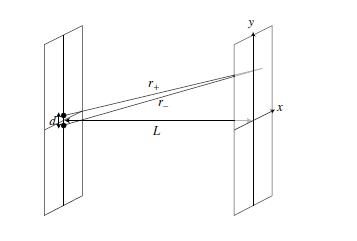
Suppose that a beam of electrons, traveling along the $z$ axis, hits a screen at $z=0\!$ with two pinholes at $x=0,y=\pm d/2\!$. For a point $(x,y)\!$ on a second screen at $z=L>>d,\lambda \!$, the distance from each pinhole is given by $r_{\pm }={\sqrt {x^{2}+(y\mp d/2)^{2}+L^{2}}}\!$. A spherical wave is emitted from each pinhole, and the waves from each add, and hence the wave function at a given point on the second screen is

$\psi (x,y)={\frac {e^{ikr_{+}}}{r_{+}}}+{\frac {e^{ikr_{-}}}{r_{-}}}$,

where $k=2\pi /\lambda \!$. Answer the following questions.

(a) Considering just the exponential factors, show that the constructive interference appears approximately at

${\frac {y}{r}}=n{\frac {\lambda }{d}}$

where $r={\sqrt {x^{2}+y^{2}+L^{2}}}$.

(b) Make a plot of the intensity $|\psi (0,y)|^{2}\!$ as a function of $y\!$, by choosing $k=1,d=20\!$, and $L=1000\!$. The intensity $|\psi (0,y)|^{2}\!$ is interpreted as the probability distribution for the electron to be detected on the screen, after repeating the same experiment many many times.

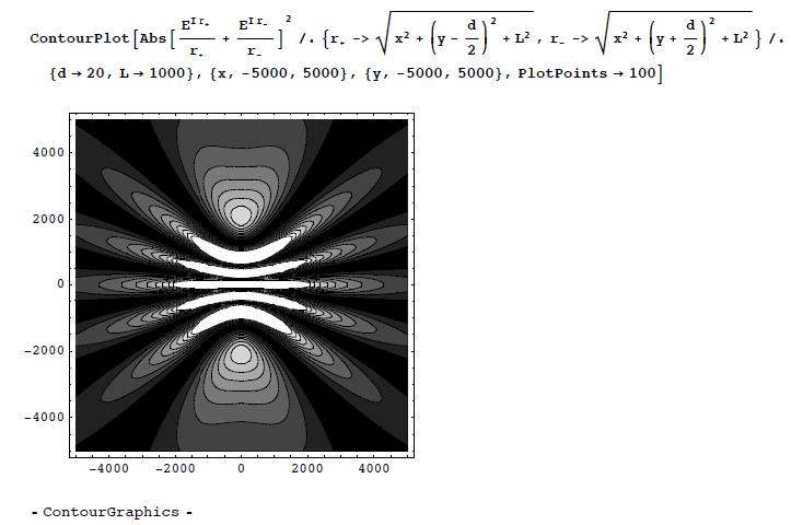
(c) Make a contour plot of the intensity $|\psi (x,y)|^{2}\!$ as afunction of x and y, for the same parameters.

(d) If you place a counter at both pinholes to see if the electron has passed one of them, all of a sudden the wave function "collapses". If the electron is observed to pass through the pinhole at $y=+d/2\!$, the wave function becomes

$\psi _{+}(x,y)={\frac {e^{ikr_{+}}}{r_{+}}}$.

If it is observed to pass through that at $y=-d/2\!$, the wave function becomes

$\psi _{-}(x,y)={\frac {e^{ikr_{-}}}{r_{-}}}$.

After repeating this experiment many times with 50:50 probability for each the pinholes, the probability on the screen will be given by

$|\psi _{+}(x,y)|^{2}+|\psi _{-}(x,y)|^{2}\!$

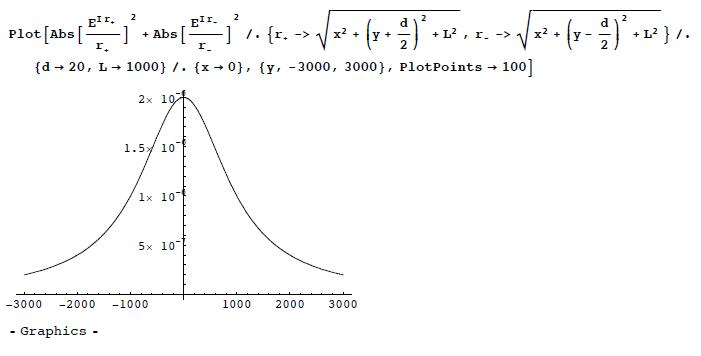
instead. Plot this function on y-axis, and also show the contour plot, to compare its pattern to the case when you do not place a counter. What is the difference from the case without the counter?

---

Answer:

(a) As directed, we assume that the denominators are approximately the same between two waves. This is justified because the corrections are only of the order of $d/l\!$, and we are interested in the case where $d<<L\!$. We require that the numerators have the same phase, namely $kr_{+}-kr_{-}=2\pi n\!$. We expand the LHS with respect to $d\!$,

Failed to parse (SVG (MathML can be enabled via browser plugin): Invalid response ("Math extension cannot connect to Restbase.") from server "https://wikimedia.org/api/rest_v1/":): {\displaystyle \begin{align} k(r_{+}-r_{-})&\approx k\left\{\left(\sqrt{L^{2}+x^{2}+y^{2}}+\frac{yd}{2\sqrt{L^{2}+x^{2}+y^{2}}}\right) \right. \\ &-\left.\left(\sqrt{L^{2}+x^{2}+y^{2}}-\frac{yd}{2\sqrt{L^{2}+x^{2}+y^{2}}}\right)\right\}\\ &=k\frac{dy}{\sqrt{L^{2}+x^{2}+y^{2}}} \end{align} }

Therefore,$k{\frac {dy}{\sqrt {L^{2}+x^{2}+y^{2}}}}=2\pi n\!$

and hence

${\frac {y}{\sqrt {L^{2}+x^{2}+y^{2}}}}=n{\frac {\lambda }{d}}\!$

(b) Let us choose the unit where k = 1. Then we pick d = 20, L = 1000. Here is the interference pattern. First along the y-axis (x = 0):

(c) Now on the plane:

(d) For the same parameter as in (b), First along the y-axis (x = 0):

Now on the plane:

The main difference is the absence of the interference pattern.