Phy5646

Welcome to the Quantum Mechanics B PHY5646 Spring 2009

Schrodinger equation. The most fundamental equation of quantum mechanics which describes the rule according to which a state Failed to parse (SVG (MathML can be enabled via browser plugin): Invalid response ("Math extension cannot connect to Restbase.") from server "https://wikimedia.org/api/rest_v1/":): {\displaystyle |\Psi\rangle} evolves in time.

This is the second semester of a two-semester graduate level sequence, the first being PHY5645 Quantum A. Its goal is to explain the concepts and mathematical methods of Quantum Mechanics, and to prepare a student to solve quantum mechanics problems arising in different physical applications. The emphasis of the courses is equally on conceptual grasp of the subject as well as on problem solving. This sequence of courses builds the foundation for more advanced courses and graduate research in experimental or theoretical physics.

The key component of the course is the collaborative student contribution to the course Wiki-textbook. Each team of students (see Phy5646 wiki-groups) is responsible for BOTH writing the assigned chapter AND editing chapters of others.

This course's website can be found here.

---

Outline of the course:

Stationary state perturbation theory in Quantum Mechanics

Very often, quantum mechanical problems cannot be solved exactly. We have seen last semester that an approximate technique can be very useful since it gives us quantitative insight into a larger class of problems which do not admit exact solutions. The technique we used last semester was WKB, which holds in the asymptotic limit Failed to parse (SVG (MathML can be enabled via browser plugin): Invalid response ("Math extension cannot connect to Restbase.") from server "https://wikimedia.org/api/rest_v1/":): {\displaystyle \hbar\rightarrow 0 } .

Perturbation theory is another very useful technique, which is also approximate, and attempts to find corrections to exact solutions in powers of the terms in the Hamiltonian which render the problem insoluble.

Typically, the (Hamiltonian) problem has the following structure

Failed to parse (SVG (MathML can be enabled via browser plugin): Invalid response ("Math extension cannot connect to Restbase.") from server "https://wikimedia.org/api/rest_v1/":): {\displaystyle \mathcal{H}=\mathcal{H}_0+\mathcal{H}'}

where Failed to parse (SVG (MathML can be enabled via browser plugin): Invalid response ("Math extension cannot connect to Restbase.") from server "https://wikimedia.org/api/rest_v1/":): {\displaystyle \mathcal{H}_0} is exactly soluble and Failed to parse (SVG (MathML can be enabled via browser plugin): Invalid response ("Math extension cannot connect to Restbase.") from server "https://wikimedia.org/api/rest_v1/":): {\displaystyle \mathcal{H}'} makes it insoluble.

Rayleigh-Schrödinger Perturbation Theory

We begin with an unperturbed problem, whose solution is known exactly. That is, for the unperturbed Hamiltonian, Failed to parse (SVG (MathML can be enabled via browser plugin): Invalid response ("Math extension cannot connect to Restbase.") from server "https://wikimedia.org/api/rest_v1/":): {\displaystyle \mathcal{H}_0} , we have eigenstates, Failed to parse (SVG (MathML can be enabled via browser plugin): Invalid response ("Math extension cannot connect to Restbase.") from server "https://wikimedia.org/api/rest_v1/":): {\displaystyle |n\rangle } , and eigenenergies, Failed to parse (SVG (MathML can be enabled via browser plugin): Invalid response ("Math extension cannot connect to Restbase.") from server "https://wikimedia.org/api/rest_v1/":): {\displaystyle \epsilon_n } , that are known solutions to the Schrodinger eq:

Failed to parse (SVG (MathML can be enabled via browser plugin): Invalid response ("Math extension cannot connect to Restbase.") from server "https://wikimedia.org/api/rest_v1/":): {\displaystyle \mathcal{H}_0 |n\rangle = \epsilon_n |n\rangle \qquad\qquad\qquad\qquad\qquad\qquad\qquad\qquad\qquad\qquad\qquad\qquad\qquad\qquad\qquad\qquad\qquad (1.1.1) }

To find the solution to the perturbed hamiltonian, Failed to parse (SVG (MathML can be enabled via browser plugin): Invalid response ("Math extension cannot connect to Restbase.") from server "https://wikimedia.org/api/rest_v1/":): {\displaystyle \mathcal{H}} , we first consider an auxiliary problem, parameterized by Failed to parse (SVG (MathML can be enabled via browser plugin): Invalid response ("Math extension cannot connect to Restbase.") from server "https://wikimedia.org/api/rest_v1/":): {\displaystyle \lambda} :

Failed to parse (SVG (MathML can be enabled via browser plugin): Invalid response ("Math extension cannot connect to Restbase.") from server "https://wikimedia.org/api/rest_v1/":): {\displaystyle \mathcal{H} = \mathcal{H}_0 + \lambda \mathcal{H}^' \qquad\qquad\qquad\qquad\qquad\qquad\qquad\qquad\qquad\qquad\qquad\qquad\qquad\qquad\qquad\qquad\qquad (1.1.2) }

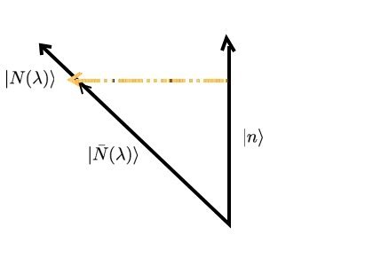
If we attempt to find eigenstates Failed to parse (SVG (MathML can be enabled via browser plugin): Invalid response ("Math extension cannot connect to Restbase.") from server "https://wikimedia.org/api/rest_v1/":): {\displaystyle |N(\lambda)\rangle} and eigenvalues Failed to parse (SVG (MathML can be enabled via browser plugin): Invalid response ("Math extension cannot connect to Restbase.") from server "https://wikimedia.org/api/rest_v1/":): {\displaystyle E_n} of the Hermitian operator Failed to parse (SVG (MathML can be enabled via browser plugin): Invalid response ("Math extension cannot connect to Restbase.") from server "https://wikimedia.org/api/rest_v1/":): {\displaystyle \mathcal{H}} , and assume that they can be expanded in a power series of Failed to parse (SVG (MathML can be enabled via browser plugin): Invalid response ("Math extension cannot connect to Restbase.") from server "https://wikimedia.org/api/rest_v1/":): {\displaystyle \lambda} :

Failed to parse (SVG (MathML can be enabled via browser plugin): Invalid response ("Math extension cannot connect to Restbase.") from server "https://wikimedia.org/api/rest_v1/":): {\displaystyle E_n(\lambda) = E_n^{(0)} + \lambda E_n^{(1)} + ... + \lambda^j E_n^{(j)} + ... |N(\lambda)\rangle = |\Psi_n^{(0)}\rangle + \lambda|\Psi_n^{(1)}\rangle + \lambda^2 |\Psi_n^{(2)}\rangle + ... \lambda^j |\Psi_n^{(j)}\rangle + ... \qquad\qquad (1.1.3)}

Where the Failed to parse (SVG (MathML can be enabled via browser plugin): Invalid response ("Math extension cannot connect to Restbase.") from server "https://wikimedia.org/api/rest_v1/":): {\displaystyle |\Psi_n^{(0)}\rangle} signify the nth order correction to the unperturbed eigenstate Failed to parse (SVG (MathML can be enabled via browser plugin): Invalid response ("Math extension cannot connect to Restbase.") from server "https://wikimedia.org/api/rest_v1/":): {\displaystyle |n\rangle} , upon perturbation. Then we must have,

Failed to parse (SVG (MathML can be enabled via browser plugin): Invalid response ("Math extension cannot connect to Restbase.") from server "https://wikimedia.org/api/rest_v1/":): {\displaystyle \mathcal{H} |N(\lambda)\rangle = E(\lambda) |N(\lambda)\rangle \qquad\qquad\qquad\qquad\qquad\qquad\qquad\qquad\qquad\qquad\qquad\qquad\qquad\qquad\qquad (1.1.4)} .

Which upon expansion, becomes:

Failed to parse (SVG (MathML can be enabled via browser plugin): Invalid response ("Math extension cannot connect to Restbase.") from server "https://wikimedia.org/api/rest_v1/":): {\displaystyle (\mathcal{H}_0 + \lambda \mathcal{H}')\left(\sum_{j=0}^{\infty}\lambda^j |\Psi_n^{(j)}\rangle \right) = \left(\sum_{l=0}^{\infty} \lambda^l E_l\right)\left(\sum_{j=0}^{\infty}\lambda^j |\Psi_n^{(j)}\rangle \right) \qquad\qquad\qquad\qquad\qquad\qquad\qquad\qquad (1.1.5)}

In order for this method to be useful, the perturbed energies must vary continuously with Failed to parse (SVG (MathML can be enabled via browser plugin): Invalid response ("Math extension cannot connect to Restbase.") from server "https://wikimedia.org/api/rest_v1/":): {\displaystyle \lambda} . Knowing this we can see several things about our, as yet undetermined perturbed energies and eigenstates. For one, as Failed to parse (SVG (MathML can be enabled via browser plugin): Invalid response ("Math extension cannot connect to Restbase.") from server "https://wikimedia.org/api/rest_v1/":): {\displaystyle \lambda \rightarrow 0, |N(\lambda)\rangle \rightarrow |n\rangle} and Failed to parse (SVG (MathML can be enabled via browser plugin): Invalid response ("Math extension cannot connect to Restbase.") from server "https://wikimedia.org/api/rest_v1/":): {\displaystyle E_n^{(0)} = \epsilon_n} for some unperturbed state Failed to parse (SVG (MathML can be enabled via browser plugin): Invalid response ("Math extension cannot connect to Restbase.") from server "https://wikimedia.org/api/rest_v1/":): {\displaystyle |n\rangle} .

For convenience, assume that the unperturbed states are already normalized: Failed to parse (SVG (MathML can be enabled via browser plugin): Invalid response ("Math extension cannot connect to Restbase.") from server "https://wikimedia.org/api/rest_v1/":): {\displaystyle \langle n | n \rangle = 1} , and choose normalization such that the exact states satisfy Failed to parse (SVG (MathML can be enabled via browser plugin): Invalid response ("Math extension cannot connect to Restbase.") from server "https://wikimedia.org/api/rest_v1/":): {\displaystyle \langle n|N(\lambda)\rangle=1} . Then in general Failed to parse (SVG (MathML can be enabled via browser plugin): Invalid response ("Math extension cannot connect to Restbase.") from server "https://wikimedia.org/api/rest_v1/":): {\displaystyle |N\rangle} will not be normalized, and we must normalize it after we have found the states. We have:

Failed to parse (SVG (MathML can be enabled via browser plugin): Invalid response ("Math extension cannot connect to Restbase.") from server "https://wikimedia.org/api/rest_v1/":): {\displaystyle \langle n|N(\lambda)\rangle= 1 = \langle n |\Psi_n^{(0)}\rangle + \lambda \langle n |\Psi_n^{(1)}\rangle + \lambda^2 \langle n |\Psi_n^{(2)}\rangle + ... \qquad\qquad\qquad\qquad\qquad\qquad\qquad\qquad\qquad(1.1.6)}

Coefficients of the powers of Failed to parse (SVG (MathML can be enabled via browser plugin): Invalid response ("Math extension cannot connect to Restbase.") from server "https://wikimedia.org/api/rest_v1/":): {\displaystyle \lambda} must match, so,

Failed to parse (SVG (MathML can be enabled via browser plugin): Invalid response ("Math extension cannot connect to Restbase.") from server "https://wikimedia.org/api/rest_v1/":): {\displaystyle \langle n | N_n^{(i)} \rangle = 0, i = 1, 2, 3, ... \qquad\qquad\qquad\qquad\qquad\qquad\qquad\qquad\qquad\qquad\qquad\qquad\qquad\qquad\qquad(1.1.7)}

Which shows that, if we start out with the unperturbed state Failed to parse (SVG (MathML can be enabled via browser plugin): Invalid response ("Math extension cannot connect to Restbase.") from server "https://wikimedia.org/api/rest_v1/":): {\displaystyle |n\rangle } , upon perturbation, the original state is added to a set of perturbation states, Failed to parse (SVG (MathML can be enabled via browser plugin): Invalid response ("Math extension cannot connect to Restbase.") from server "https://wikimedia.org/api/rest_v1/":): {\displaystyle |\Psi_n^{(0)}\rangle, |\Psi_n^{(1)}\rangle, ... } which are all orthogonal to the original state.

If we equate coefficients in the above expanded form of the perturbed Hamiltonian, we are provided with the corrected eigenvalues for whichever order of Failed to parse (SVG (MathML can be enabled via browser plugin): Invalid response ("Math extension cannot connect to Restbase.") from server "https://wikimedia.org/api/rest_v1/":): {\displaystyle \lambda} that we want. The first few are as follows,

0th Order Energy Failed to parse (SVG (MathML can be enabled via browser plugin): Invalid response ("Math extension cannot connect to Restbase.") from server "https://wikimedia.org/api/rest_v1/":): {\displaystyle \lambda = 0 \rightarrow E_n^{(0)} = \epsilon_n } , which we already had from before (1.1.8)

1st Order Energy Corrections Failed to parse (SVG (MathML can be enabled via browser plugin): Invalid response ("Math extension cannot connect to Restbase.") from server "https://wikimedia.org/api/rest_v1/":): {\displaystyle \lambda = 1 \rightarrow \mathcal{H}_0 |\Psi_n^{(1)}\rangle + \mathcal{H}' |\Psi_n^{(0)}\rangle = E_n^{(1)} |\Psi_n^{(0)}\rangle + E_n^{(0)} |\Psi_n^{(1)}\rangle } , taking the scalar product of this result of Failed to parse (SVG (MathML can be enabled via browser plugin): Invalid response ("Math extension cannot connect to Restbase.") from server "https://wikimedia.org/api/rest_v1/":): {\displaystyle |n\rangle} , and using our previous results, we get: Failed to parse (SVG (MathML can be enabled via browser plugin): Invalid response ("Math extension cannot connect to Restbase.") from server "https://wikimedia.org/api/rest_v1/":): {\displaystyle E_n^{(1)} = \langle n|\mathcal{H}'|n\rangle }

kth order Energy Corrections In general, Failed to parse (SVG (MathML can be enabled via browser plugin): Invalid response ("Math extension cannot connect to Restbase.") from server "https://wikimedia.org/api/rest_v1/":): {\displaystyle E_n^{(k)} = \langle n | \mathcal{H}' | N_n^{(k - 1)} \rangle \qquad\qquad\qquad\qquad\qquad\qquad\qquad\qquad(1.1.9)}

This result provides us with a recursive relationship for the Eigenenergies of the perturbed state, so that we have access to the eigenenergies for an state of arbitrary order in Failed to parse (SVG (MathML can be enabled via browser plugin): Invalid response ("Math extension cannot connect to Restbase.") from server "https://wikimedia.org/api/rest_v1/":): {\displaystyle \lambda} .

What about the eigenstates? Express the perturbed states in terms of the unperturbed states:

Failed to parse (SVG (MathML can be enabled via browser plugin): Invalid response ("Math extension cannot connect to Restbase.") from server "https://wikimedia.org/api/rest_v1/":): {\displaystyle |\Psi_n^{(k)}\rangle = \sum_{m \not= n}|m\rangle\langle m|\Psi^{(k)}\rangle}

Go back to equation 1.1.5 and taking the scalar product from the left with Failed to parse (SVG (MathML can be enabled via browser plugin): Invalid response ("Math extension cannot connect to Restbase.") from server "https://wikimedia.org/api/rest_v1/":): {\displaystyle \langle m |} and taking orders of Failed to parse (SVG (MathML can be enabled via browser plugin): Invalid response ("Math extension cannot connect to Restbase.") from server "https://wikimedia.org/api/rest_v1/":): {\displaystyle \lambda} we find:

1th order Eigenkets

Failed to parse (SVG (MathML can be enabled via browser plugin): Invalid response ("Math extension cannot connect to Restbase.") from server "https://wikimedia.org/api/rest_v1/":): {\displaystyle \langle m|\Psi_n^{(1)}\rangle = \frac{\langle m | n\rangle}{\epsilon_n - \epsilon_m}}

The first order contribution is then the sum of this equation over all Failed to parse (SVG (MathML can be enabled via browser plugin): Invalid response ("Math extension cannot connect to Restbase.") from server "https://wikimedia.org/api/rest_v1/":): {\displaystyle m} , and adding the zeroth order we get the eigenstates of the perturbed hamiltonian to the 1st order in Failed to parse (SVG (MathML can be enabled via browser plugin): Invalid response ("Math extension cannot connect to Restbase.") from server "https://wikimedia.org/api/rest_v1/":): {\displaystyle \lambda} :

Failed to parse (SVG (MathML can be enabled via browser plugin): Invalid response ("Math extension cannot connect to Restbase.") from server "https://wikimedia.org/api/rest_v1/":): {\displaystyle |N\rangle = |n\rangle + \lambda\sum_{k \not= n} |m\rangle \frac{\langle m |V| n\rangle}{\epsilon_n - \epsilon_m} \qquad\qquad\qquad\qquad\qquad\qquad\qquad\qquad\qquad\qquad\qquad\qquad\qquad(1.1.7)}

Renormalization Earlier we assumed that Failed to parse (SVG (MathML can be enabled via browser plugin): Invalid response ("Math extension cannot connect to Restbase.") from server "https://wikimedia.org/api/rest_v1/":): {\displaystyle \langle n|N(\lambda)\rangle=1} , which means that our Failed to parse (SVG (MathML can be enabled via browser plugin): Invalid response ("Math extension cannot connect to Restbase.") from server "https://wikimedia.org/api/rest_v1/":): {\displaystyle |N(\lambda)\rangle} states are not normalized themselves. To reconsile this we introduce the normalized perturbed eigenstates, denoted Failed to parse (SVG (MathML can be enabled via browser plugin): Invalid response ("Math extension cannot connect to Restbase.") from server "https://wikimedia.org/api/rest_v1/":): {\displaystyle bar{N}} . These will then be related to the $N(\lambda )<math>:<math>|{\bar {N}}\rangle ={\frac {|N\rangle }{\langle N|N\rangle }}=z\qquad \qquad \qquad \qquad \qquad \qquad \qquad \qquad \qquad \qquad \qquad (1.1.10)$

Thus $z$ gives us a measure of how close the perturbed state is to the original state.

$z={\frac {1}{\langle N|N\rangle }}\qquad \qquad \qquad \qquad \qquad \qquad \qquad \qquad \qquad \qquad \qquad \qquad \qquad \qquad \qquad \qquad \qquad \qquad \qquad (1.1.11)$

To 2nd order in $\lambda$

${\frac {1}{z}}=\langle N|N\rangle =(\langle n|+\lambda \langle \Psi _{n}^{(1)}|+...)(|n\rangle +|\Psi _{n}^{(1)}\rangle +...)$

$z={\frac {1}{1+\lambda ^{2}\sum _{n\not =m}{\frac {|\langle m|V|n\rangle |^{2}}{(\epsilon _{n}-\epsilon _{m})^{2}}}+...}}=1-\lambda ^{2}\sum _{n\not =m}{\frac {|\langle m|V|n\rangle |^{2}}{(\epsilon _{n}-\epsilon _{m})^{2}}}+...$

Where we use a taylor expansion to arrive at the final result (noting that ${\frac {|\langle m|V|n\rangle |^{2}}{(\epsilon _{n}-\epsilon _{m})^{2}}}<1$).

We can show that $|n\rangle$ is related to the energies by employing equation 1.1.9:

$z={\frac {\partial E_{n}}{\partial \epsilon _{n}}}{\Big |}_{\epsilon _{m}:\langle m|V|n>}$

Brillouin-Wigner Perturbation Theory

This is another type of perturbation theory. Using a basic formula derived from the Schroedinger equation, you can find an approximation for any power of $\lambda$ required using an iterative process. Starting with the Schroedinger equation:

${\begin{aligned}({\mathcal {H}}_{o}+\lambda {\mathcal {H}}')|N\rangle &=E_{n}|N\rangle \\\lambda {\mathcal {H}}'|N\rangle &=(E_{n}-{\mathcal {H}}_{o})|N\rangle \\\langle n|(\lambda {\mathcal {H}}'|N\rangle )&=\langle n|(E_{n}-{\mathcal {H}}_{o})|N\rangle \\\lambda \langle n|{\mathcal {H}}'|N\rangle &=(E_{n}-\epsilon _{n})\langle n|N\rangle \\\end{aligned}}$

If we choose to normalize $\langle n|N\rangle =1$, then so far we have: $(E_{n}-\epsilon _{m})=\lambda \langle n|{\mathcal {H}}'|N\rangle$, which is still an exact expression (no approximation have been made yet). The wavefunction we are interested in, $|N\rangle$ can be rewritten as a summation of the eigenstates of the (unperturbed, ${\mathcal {H}}_{o}$) Hamiltonian:

${\begin{aligned}|N\rangle &=\sum _{m}|m\rangle \langle m|N\rangle \\&=|n\rangle \langle n|N\rangle +\sum _{m\neq n}|m\rangle \langle m|N\rangle \\&=|n\rangle +\sum _{m\neq n}|m\rangle {\frac {\lambda \langle m|{\mathcal {H}}'|N\rangle }{(E_{n}-\epsilon _{m})}}\\\end{aligned}}$

So now we have a recursive relationship for both $E_{n}$ and $|N\rangle$

$E_{n}=\epsilon _{n}+\lambda \langle n|{\mathcal {H}}'|N\rangle$ where $|N\rangle$ can be written recursively to any order of $\lambda$ desired

$|N\rangle =|n\rangle +\lambda \sum _{m\neq n}|m\rangle {\frac {\lambda \langle m|{\mathcal {H}}'|N\rangle }{(E_{n}-\epsilon _{m})}}$ where $E_{n}$ can be written recursively to any order of $\lambda$ desired

For example, the expression for $|N\rangle$ to a third order in $\lambda$ would be:

${\begin{aligned}|N\rangle &=|n\rangle +\lambda \sum _{m\neq n}|m\rangle {\frac {\langle m|{\mathcal {H}}'}{(E_{n}-\epsilon _{m})}}\left(|n\rangle +\lambda \sum _{j\neq n}|j\rangle {\frac {\langle j|{\mathcal {H}}'}{(E_{n}-\epsilon _{j})}}\left(|n\rangle +\lambda \sum _{k\neq n}|k\rangle {\frac {\langle k|{\mathcal {H}}'|n\rangle }{(E_{n}-\epsilon _{k})}}\right)\right)\\&=|n\rangle +\lambda \sum _{m\neq n}|m\rangle {\frac {\langle m|{\mathcal {H}}'|n\rangle }{(E_{n}-\epsilon _{m})}}+\lambda ^{2}\sum _{m,j\neq n}|m\rangle {\frac {\langle m|{\mathcal {H}}'|j\rangle \langle j|{\mathcal {H}}'|n\rangle }{(E_{n}-\epsilon _{m})(E_{n}-\epsilon _{j})}}+\lambda ^{3}\sum _{m,j,k\neq n}|m\rangle {\frac {\langle m|{\mathcal {H}}'|j\rangle \langle j|{\mathcal {H}}'|k\rangle \langle k|{\mathcal {H}}'|n\rangle }{(E_{n}-\epsilon _{m})(E_{n}-\epsilon _{j})(E_{n}-\epsilon _{k})}}\\\end{aligned}}$

where $\sum _{j}|j\rangle \langle j|$ is unity

Note that we have chosen $\langle n|N\rangle =1$, i.e. the correction is perpendicular to the unperturbed state. That is why at this point $|N\rangle$ is not normalized. The normalized exact state, therefore, is written as $Z|N\rangle$. Interestingly, the normalization constant $Z$ turns out be exactly equal to the derivative of the exact energy with respect to the unperturbed energy. The calculation for the normalization constant can be found through this link

Degenerate Perturbation Theory

If more than one eigenstate for the Hamiltonian ${\mathcal {H}}_{o}$ has the same energy value, the problem is said to be degenerate. If we try to get a solution using perturbation theory, we fail, since Rayleigh-Schroedinger PT includes terms like $1/(\epsilon _{n}-\epsilon _{m})$.

Instead of trying to use these (degenerate) eigenstates with perturbation theory, if we start with the correct linear combinations of eigenstates, regular perturbation theory will no longer fail! So the issue now is how to find these linear combinations.

Failed to parse (SVG (MathML can be enabled via browser plugin): Invalid response ("Math extension cannot connect to Restbase.") from server "https://wikimedia.org/api/rest_v1/":): {\displaystyle \{|n_a\rangle,|n_b\rangle,|n_c\rangle,\dots\} } Failed to parse (SVG (MathML can be enabled via browser plugin): Invalid response ("Math extension cannot connect to Restbase.") from server "https://wikimedia.org/api/rest_v1/":): {\displaystyle \longrightarrow } Failed to parse (SVG (MathML can be enabled via browser plugin): Invalid response ("Math extension cannot connect to Restbase.") from server "https://wikimedia.org/api/rest_v1/":): {\displaystyle \{|n_{\alpha}\rangle,|n_{\beta}\rangle,|n_{\gamma}\rangle,\dots\} } where Failed to parse (SVG (MathML can be enabled via browser plugin): Invalid response ("Math extension cannot connect to Restbase.") from server "https://wikimedia.org/api/rest_v1/":): {\displaystyle |n_{\alpha}\rangle = \sum_iC_{\alpha,i}|n_i\rangle } etc

The general procedure for doing this type of problem is to create the matrix with elements Failed to parse (SVG (MathML can be enabled via browser plugin): Invalid response ("Math extension cannot connect to Restbase.") from server "https://wikimedia.org/api/rest_v1/":): {\displaystyle \langle n_a|{\mathcal H}'|n_b\rangle } formed from the degenerate eigenstates of Failed to parse (SVG (MathML can be enabled via browser plugin): Invalid response ("Math extension cannot connect to Restbase.") from server "https://wikimedia.org/api/rest_v1/":): {\displaystyle {\mathcal H}_o } . This matrix can then be diagonalized, and the eigenstates of this matrix are the correct linear combinations to be used in non-degenerate perturbation theory.

One of the well-known examples of an application of degenerate perturbation theory is the Stark Effect. If we consider a Hydrogen atom with Failed to parse (SVG (MathML can be enabled via browser plugin): Invalid response ("Math extension cannot connect to Restbase.") from server "https://wikimedia.org/api/rest_v1/":): {\displaystyle n=2 } in the presence of an external electric field Failed to parse (SVG (MathML can be enabled via browser plugin): Invalid response ("Math extension cannot connect to Restbase.") from server "https://wikimedia.org/api/rest_v1/":): {\displaystyle \vec{\mathcal E}={\mathcal E}\hat{z} } . The Hamiltonian for this system is Failed to parse (SVG (MathML can be enabled via browser plugin): Invalid response ("Math extension cannot connect to Restbase.") from server "https://wikimedia.org/api/rest_v1/":): {\displaystyle {\mathcal H}={\mathcal H}_o-e{\mathcal E}z } . The eigenstates of the system are Failed to parse (SVG (MathML can be enabled via browser plugin): Invalid response ("Math extension cannot connect to Restbase.") from server "https://wikimedia.org/api/rest_v1/":): {\displaystyle \{|2S\rangle,|2P_{-1}\rangle,|2P_0\rangle,|2P_{+1}\rangle\} } . The matrix of the degenerate eigenstates and the perturbation is:

Failed to parse (SVG (MathML can be enabled via browser plugin): Invalid response ("Math extension cannot connect to Restbase.") from server "https://wikimedia.org/api/rest_v1/":): {\displaystyle \begin{align} \langle n_i|{\mathcal H}'|n_j\rangle &\longrightarrow \left(\begin{array}{cccc}\langle2S|-e{\mathcal E}z|2S\rangle&\langle2S|-e{\mathcal E}z|2P_{-1}\rangle&\langle2S|-e{\mathcal E}z|2P_0\rangle&\langle2S|-e{\mathcal E}z|2P_{+1}\rangle\\\langle2P_{-1}|-e{\mathcal E}z|2S\rangle&\langle2P_{-1}|-e{\mathcal E}z|2P_{-1}\rangle&\langle2P_{-1}|-e{\mathcal E}z|2P_0\rangle&\langle2P_{-1}|-e{\mathcal E}z|2P_{+1}\rangle\\\langle2P_0|-e{\mathcal E}z|2S\rangle&\langle2P_0|-e{\mathcal E}z|2P_{-1}\rangle&\langle2P_0|-e{\mathcal E}z|2P_0\rangle&\langle2P_0|-e{\mathcal E}z|2P_{+1}\rangle\\\langle2P_{+1}|-e{\mathcal E}z|2S\rangle&\langle2P_{+1}|-e{\mathcal E}z|2P_{-1}\rangle&\langle2P_{+1}|-e{\mathcal E}z|2P_0\rangle&\langle2P_{+1}|-e{\mathcal E}z|2P_{+1}\rangle\\\end{array}\right)\\ &\longrightarrow \left(\begin{array}{cccc}0&0&\langle2S|-e{\mathcal E}z|2P_0\rangle&0\\0&0&0&0\\\langle2P_0|-e{\mathcal E}z|2S\rangle&0&0&0\\0&0&0&0\\\end{array}\right)\\ &\longrightarrow \left(\begin{array}{cccc}0&0&-3e{\mathcal E}a_B&0\\0&0&0&0\\-3e{\mathcal E}a_B&0&0&0\\0&0&0&0\\\end{array}\right)\\ \end{align} }

The full arguments as to how most of these terms are zero is worked out in G Baym's "Lectures on Quantum Mechanics" in the section on Degenerate Perturbation Theory. The correct linear combination of the degenerate eigenstates ends up being

Failed to parse (SVG (MathML can be enabled via browser plugin): Invalid response ("Math extension cannot connect to Restbase.") from server "https://wikimedia.org/api/rest_v1/":): {\displaystyle \{|2P_{-1}\rangle,|2P_{+1}\rangle,\frac{1}{\sqrt{2}}\left(|2S\rangle+|2P_0\rangle\right),\frac{1}{\sqrt{2}}\left(|2S\rangle-|2P_0\rangle\right)\} }

Because of the perturbation due to the electric field, the Failed to parse (SVG (MathML can be enabled via browser plugin): Invalid response ("Math extension cannot connect to Restbase.") from server "https://wikimedia.org/api/rest_v1/":): {\displaystyle |2P_{-1}\rangle } and Failed to parse (SVG (MathML can be enabled via browser plugin): Invalid response ("Math extension cannot connect to Restbase.") from server "https://wikimedia.org/api/rest_v1/":): {\displaystyle |2P_{+1}\rangle } states will be unaffected. However, the energy of the Failed to parse (SVG (MathML can be enabled via browser plugin): Invalid response ("Math extension cannot connect to Restbase.") from server "https://wikimedia.org/api/rest_v1/":): {\displaystyle |2S\rangle } and Failed to parse (SVG (MathML can be enabled via browser plugin): Invalid response ("Math extension cannot connect to Restbase.") from server "https://wikimedia.org/api/rest_v1/":): {\displaystyle |2P_0\rangle } states will have a shift due to the electric field.

Time dependent perturbation theory in Quantum Mechanics

Formalism

Previously, we learned the time independent perturbation theory which can be applied on various systems in which a little change in the Hamiltonian appears as a
correction in the form of a series for the energy and wave functions. However, this stationary approach cannot be used to describe the interaction of electromagnetic field
with atoms i.e. photon with Hydrogen atom. This leads us to the Time Dependent Perturbation Theory.

One of the main tasks of this theory is the calculation of transition probabilities from one state Failed to parse (SVG (MathML can be enabled via browser plugin): Invalid response ("Math extension cannot connect to Restbase.") from server "https://wikimedia.org/api/rest_v1/":): {\displaystyle |\psi_n \rangle} to another state Failed to parse (SVG (MathML can be enabled via browser plugin): Invalid response ("Math extension cannot connect to Restbase.") from server "https://wikimedia.org/api/rest_v1/":): {\displaystyle |\psi_m \rangle} that occurs under the influence of time
dependent potential. Generally, transition of a system from one state to another state only makes sense if the potential acts only within a finite time period from Failed to parse (SVG (MathML can be enabled via browser plugin): Invalid response ("Math extension cannot connect to Restbase.") from server "https://wikimedia.org/api/rest_v1/":): {\displaystyle \!t = 0}
to Failed to parse (SVG (MathML can be enabled via browser plugin): Invalid response ("Math extension cannot connect to Restbase.") from server "https://wikimedia.org/api/rest_v1/":): {\displaystyle \!t = T} . Except for this time period, the total energy is a constant of motion which can be measured. We start with the Time Dependent Schrodinger Equation

Failed to parse (SVG (MathML can be enabled via browser plugin): Invalid response ("Math extension cannot connect to Restbase.") from server "https://wikimedia.org/api/rest_v1/":): {\displaystyle i\hbar\frac{\partial}{\partial t}|\psi_t^0 \rangle = H_0 |\psi_t^0\rangle, \qquad t<t_0 \qquad \qquad \qquad \qquad \qquad \qquad \qquad \qquad \qquad \qquad \qquad \qquad \qquad \qquad \qquad \qquad \qquad \qquad (2.1)}

then assuming that the perturbation acts after time Failed to parse (SVG (MathML can be enabled via browser plugin): Invalid response ("Math extension cannot connect to Restbase.") from server "https://wikimedia.org/api/rest_v1/":): {\displaystyle \!t_0} , we get

Failed to parse (SVG (MathML can be enabled via browser plugin): Invalid response ("Math extension cannot connect to Restbase.") from server "https://wikimedia.org/api/rest_v1/":): {\displaystyle i\hbar\frac{\partial}{\partial t}|\psi_t \rangle = (H_0 + V_t)|\psi_t\rangle, \qquad t>t_0 \qquad \qquad \qquad \qquad \qquad \qquad \qquad \qquad \qquad \qquad \qquad \qquad \qquad \qquad \qquad \qquad \quad\;\;\; (2.2)}

The problem therefore consists of finding the solution Failed to parse (SVG (MathML can be enabled via browser plugin): Invalid response ("Math extension cannot connect to Restbase.") from server "https://wikimedia.org/api/rest_v1/":): {\displaystyle |\psi(t)\rangle} with boundary condition Failed to parse (SVG (MathML can be enabled via browser plugin): Invalid response ("Math extension cannot connect to Restbase.") from server "https://wikimedia.org/api/rest_v1/":): {\displaystyle |\psi(t)\rangle = |\psi_t^0\rangle} for Failed to parse (SVG (MathML can be enabled via browser plugin): Invalid response ("Math extension cannot connect to Restbase.") from server "https://wikimedia.org/api/rest_v1/":): {\displaystyle t \leq t_0} . However, such a problem is not generally soluble.
Therefore, we limit ourselves to the problems in which Failed to parse (SVG (MathML can be enabled via browser plugin): Invalid response ("Math extension cannot connect to Restbase.") from server "https://wikimedia.org/api/rest_v1/":): {\displaystyle \!V_t} is small.

Since Failed to parse (SVG (MathML can be enabled via browser plugin): Invalid response ("Math extension cannot connect to Restbase.") from server "https://wikimedia.org/api/rest_v1/":): {\displaystyle \!V_t} is small, the time dependence of the solution will largely come from $\!H_{0}$. So we use

$|\psi _{t}\rangle =e^{-iH_{0}t/\hbar }|\psi (t)\rangle \qquad \qquad \qquad \qquad \qquad \qquad \qquad \qquad \qquad \qquad \qquad \qquad \qquad \qquad \qquad \qquad \qquad \qquad \qquad \qquad \;(2.3)$

Which we substitute into the Schrodinger Equation to get

$i\hbar {\frac {\partial }{\partial t}}|\psi (t)\rangle =V(t)|\psi (t)\rangle \quad {\text{where}}\quad V(t)=e^{iH_{0}t/\hbar }V_{t}e^{-iH_{0}t/\hbar }\qquad \qquad \qquad \qquad \qquad \qquad \qquad \qquad \qquad \qquad \qquad \qquad (2.4)$

In this equation we work using interaction representation. Now, we integrate equation #(2.4) to get

$\int _{t_{o}}^{t}dt{\frac {\partial }{\partial t}}|\psi (t)\rangle =\psi (t)-\psi (t_{0})={\frac {1}{i\hbar }}\int _{t_{0}}^{t}dt'V(t')|\psi (t')\rangle$

or

$|\psi (t)\rangle =|\psi (t_{0})\rangle +{\frac {1}{i\hbar }}\int _{t_{0}}^{t}dt'V(t')|\psi (t')\rangle \qquad \qquad \qquad \qquad \qquad \qquad \qquad \qquad \qquad \qquad \qquad \qquad \qquad \qquad \qquad \qquad \;\;\ (2.5)$

Equation #(2.5) can be iterated by inserting this equation itself as the integrand in the r.h.s. We can then write equation #(2.5) as

$|\psi (t)\rangle =|\psi (t_{0})\rangle +{\frac {1}{i\hbar }}\int _{t_{0}}^{t}dt'V(t')\left(|\psi (t_{0})\rangle +{\frac {1}{i\hbar }}\int _{t_{0}}^{t}dt''V(t'')|\psi (t'')\rangle \right),\qquad t''<t'\qquad \qquad \qquad \qquad \qquad \qquad \qquad \quad \;\ (2.6)$

which can be written compactly as

$|\psi (t)\rangle =Te^{{\frac {i}{t}}\int _{t_{0}}^{t}V(t')dt'}\qquad \qquad \qquad \qquad \qquad \qquad \qquad \qquad \qquad \qquad \qquad \qquad \qquad \qquad \qquad \qquad \qquad \qquad \qquad \quad \;\;\ (2.7)$

With T as the time ordering operator to ensure it can be expanded in series in the correct order. For now, we consider only the correction to the first order in $\!V(t)$. If we
limit ourselves to the first order we use

$|\psi (t)\rangle =|\psi (t_{0})\rangle +{\frac {1}{i\hbar }}\int _{t_{0}}^{t}dt'V(t')|\psi (t_{0})\rangle \qquad \qquad \qquad \qquad \qquad \qquad \qquad \qquad \qquad \qquad \qquad \qquad \qquad \qquad \qquad \qquad \;\;\ (2.8)$

We want to see the system undergoes a transition to another state, say $|n\rangle$. So we project the wave function $|\psi (t)\rangle$ to $|n\rangle$. From now on, let $|\psi (t_{0})\rangle =|0\rangle$
for brevity. Projecting into state $|n\rangle$ and assuming $\langle n|0\rangle =0$ we get, ${\begin{aligned}\langle n|\psi (t)\rangle &=\langle n|0\rangle +{\frac {1}{i\hbar }}\int _{t_{0}}^{t}dt'\langle n|V(t')|0\rangle \\&={\frac {1}{i\hbar }}\int _{t_{0}}^{t}dt'\langle n|e^{{\frac {1}{\hbar }}H_{0}t}V_{t'}e^{-{\frac {1}{\hbar }}H_{0}t}|0\rangle \\&={\frac {1}{i\hbar }}\int _{t_{0}}^{t}dt'e^{{\frac {i}{\hbar }}(\epsilon _{n}-\epsilon _{0})t'}\langle n|V_{t'}|0\rangle \end{aligned}}\qquad \qquad \qquad \qquad \qquad \qquad \qquad \qquad \qquad \qquad \qquad \qquad \qquad \qquad \qquad \quad \;\,\ (2.9)$

Expression #(2.9) is the probability amplitude of transition. Therefore, we square the final expression to get the probability of having the system in state $|n\rangle$ at time t.
Squaring, we get

${\underset {0\rightarrow n}{P(t)}}=|\langle n|\psi (t)\rangle |^{2}=\left|{\frac {1}{i\hbar }}\int _{t_{0}}^{t}dt'e^{{\frac {i}{\hbar }}(\epsilon _{n}-\epsilon _{0})t'}\langle n|V_{t'}|0\rangle \right|^{2}\qquad \qquad \qquad \qquad \qquad \qquad \qquad \qquad \qquad \qquad \qquad \qquad \qquad \quad \,(2.10)$

For example, let us consider a potential $\!V_{t}$ which is turned on sharply at time $\!t_{0}$, but independent of t thereafter. Furthermore, we let $\!t_{0}=0$ for convenience. Therefore :

$V_{t}={\begin{cases}0&{\mbox{if}}\qquad t<0\\V&{\mbox{if}}\qquad t>0\end{cases}}$ ${\begin{aligned}{\underset {0\rightarrow n}{P(t)}}&=\left|{\frac {1}{i\hbar }}\int _{0}^{t}dt'e^{{\frac {i}{\hbar }}(\epsilon _{n}-\epsilon _{0})t'}\langle n|V|0\rangle \right|^{2}\\&=\left|{\frac {1}{i\hbar }}{\frac {e^{{\frac {i}{\hbar }}(\epsilon _{n}-\epsilon _{0})t'}}{{\frac {i}{\hbar }}(\epsilon _{n}-\epsilon _{0})}}\langle n|V|0\rangle \right|^{2}\\&={\frac {sin^{2}\left({\frac {\epsilon _{n}-\epsilon _{0}}{2\hbar }}t\right)}{\left({\frac {\epsilon _{n}-\epsilon _{0}}{2}}\right)^{2}}}|\langle n|V|0\rangle |^{2}\end{aligned}}\qquad \qquad \qquad \qquad \qquad \qquad \qquad \qquad \qquad \qquad \qquad \qquad \qquad \qquad \qquad \qquad \quad \;\;(2.11)$

The plot of the probability vs. $\!\epsilon _{n}$ is given as

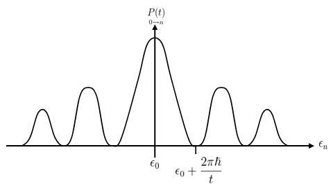
with $\Delta \epsilon \Delta t\geq 2\pi \hbar$ so we conclude that as the time grows, the probability is the largest for the transition to conserve the energy to within an amount given in that relation.

Now, we imagine shining a light of a certain frequency on a Hydrogen atom. We probably ended up getting the atom at a certain bound state. However it might be ionized as
well. The problem with ionization is the fact that the final state is a continuum, so we cannot just simply pick up a state to end with i.e. a plane wave with a specific k.
Furthermore, if the wave function is normalized, we will have a factor $1/{\sqrt {V}}$ which goes to zero if V is very large, but we know that ionization exists. So what we do is to
measure the final state from k to k+dk.

Let's suppose that the state $|n\rangle$ is one of the continuum state, then what we could ask is the probability that the system makes transition to a small group of states about
$|n\rangle$, not to a specific value of $|n\rangle$. For example, for a free particle, what we can find is the transition probability from initial state to a small group of states, viz. $|{\vec {k}}\rangle$, or in
other words the transition probability to an element of phase space $\!d^{3}k/(2\pi )^{3}$

The next step is a mathematical trick. We use

$\delta (x)=\lim _{\eta \to 0}{\frac {1}{\pi x}}sin(x/\eta )$

to derive a relation

${\frac {\pi }{\hbar }}\delta ({\frac {\epsilon _{n}-\epsilon _{0}}{2\hbar }})={\frac {sin({\frac {\epsilon _{n}-\epsilon _{0}}{2\hbar }}t)}{\frac {\epsilon _{n}-\epsilon _{0}}{2}}}\qquad \qquad \qquad \qquad \qquad \qquad \qquad \qquad \qquad \qquad \qquad \qquad \qquad \qquad \qquad \qquad \qquad \qquad \;\;\;\;\;(2.12)$

Which, if used in the equation #(2.11) gives

${\underset {0\rightarrow n}{P(t)}}\quad {\underset {t\rightarrow \infty }{\longrightarrow }}\quad {\frac {t}{\hbar }}2\pi \delta (\epsilon _{n}-\epsilon _{0})|\langle n|V|0\rangle |^{2}\qquad \qquad \qquad \qquad \qquad \qquad \qquad \qquad \qquad \qquad \qquad \qquad \qquad \qquad \qquad \qquad \quad \;(2.13)$

or as a rate of transition, ${\underset {0\rightarrow n}{\Gamma }}$ :

${\underset {0\rightarrow n}{\Gamma }}={\frac {d}{dt}}{\underset {0\rightarrow n}{P(t)}}\quad {\underset {t\rightarrow \infty }{\longrightarrow }}\quad {\frac {2\pi }{\hbar }}\delta (\epsilon _{n}-\epsilon _{0})|\langle n|V|0\rangle |^{2}\qquad \qquad \qquad \qquad \qquad \qquad \qquad \qquad \qquad \qquad \qquad \qquad \qquad \qquad \qquad (2.14)$

which is The Fermi Golden Rule. Using this formula, we should keep in mind to sum over all (continuum) final states.

To make things clear, let's try to calculate the transition probability for a system from a state $|{\vec {k}}\rangle$ to a final state $|{\vec {k'}}\rangle$ due to a potential $\!V(r)$

$\langle {\vec {k'}}|V|{\vec {k}}\rangle =\int d^{3}r{\frac {e^{-i{\vec {k'}}.{\vec {r}}}}{\sqrt {L^{3}}}}V(r){\frac {e^{i{\vec {k}}.{\vec {r}}}}{\sqrt {L^{3}}}}={\frac {V_{k'k}}{L^{3}}}\qquad \qquad \qquad \qquad \qquad \qquad \qquad \qquad \qquad \qquad \qquad \qquad \qquad \qquad \qquad \quad \;\ (2.15)$

${\underset {{\vec {k}}\rightarrow {\vec {k'}}}{\Gamma }}={\frac {2\pi }{\hbar }}\delta (\epsilon _{k}-\epsilon _{k'}){\frac {|V_{k'k}|^{2}}{L^{6}}}$

What we want is the rate of transition, or actually scattering in this case, $\!d\Gamma$ into a small solid angle $\!d\Omega$. So, we must calculate

$\sum _{k'\in d\Omega }{\underset {{\vec {k}}\rightarrow {\vec {k'}}}{\Gamma }}$

The sum over states for continuum can be calculated using integral

$\sum _{{\vec {k'}}\in d\Omega '}\quad \longrightarrow \quad d\Omega '\int d\epsilon _{k'}{\frac {L^{3}mk'}{(2\pi )^{3}\hbar ^{2}}}\qquad \qquad \qquad \qquad \qquad \qquad \qquad \qquad \qquad \qquad \qquad \qquad \qquad \qquad \qquad \qquad \qquad \;\;\ (2.16)$

Therefore,

${\underset {{\vec {k}}{k'\in d\Omega '}}{d\Gamma }}={\frac {d\Omega '}{L^{3}}}{\frac {mk}{4\pi ^{2}\hbar ^{3}}}|V_{k'k}|^{2}\qquad \qquad \qquad \qquad \qquad \qquad \qquad \qquad \qquad \qquad \qquad \qquad \qquad \qquad \qquad \qquad \qquad \qquad \quad \;\;\;\ (2.17)$

The flux of particles per incident particle of momentum $\hbar k$ in a volume $\!L^{3}$ is $\hbar k/mL^{3}$, so

${\frac {d\Gamma }{d\Omega ({\frac {\bar {k}}{mL^{3}}})}}={\frac {m^{2}}{4\pi ^{2}\hbar ^{4}}}|V_{k'k}|^{2}={\frac {d\sigma }{d\Omega }}$, in Born Approximation

This result makes sense since our potential does not depend on time, so what happened here is that we sent a particle with wave vector ${\vec {k}}$ through a potential and later detect
a particle coming out from that potential with wave vector ${\vec {k'}}$. So, it is a scattering problem solved using a different method.

Harmonic Perturbation Theory

Harmonic perturbation is one of the main interest in perturbation theory. We know that in experiment, we usually perturb the system using a certain signal to extract information about it, for example the difference between the energy levels. We could send a photon with a certain frequency to a Hydrogen atom to excite the electron and let it decay to observe the difference between two energy levels by measuring the frequency of the photon emitted from it. The photon acts as an electromagnetic signal, and it is harmonic (if we consider it as an electromagnetic wave).

In general, we write down the harmonic perturbation as

$\!V_{t}=Vcos(\omega t)e^{\eta t}\qquad \qquad \qquad \qquad \qquad \qquad \qquad \qquad \qquad \qquad \qquad \qquad \qquad \qquad \qquad \qquad (2.2.1)$

where $\!e^{\eta t}$ specify the rate at which the perturbation is turned on, $\eta$ is a very small positive number which at the end of the calculation is set to be zero.

We start from $\!t_{0}=-\infty$. Since there's no perturbation at that time, then

$\!\langle n|\psi _{t}\rangle =\langle n|e^{{\frac {-i}{\hbar }}H_{0}t}|\psi (t)\rangle =e^{{\frac {-i}{\hbar }}\epsilon _{n}t}\langle n|\psi (t)\rangle \qquad \qquad \qquad \qquad \qquad \qquad \qquad \qquad \qquad \qquad \quad (2.2.2)$

To the first order of V we write

${\begin{aligned}\langle n|\psi (t)\rangle &={\frac {1}{i\hbar }}\int _{-\infty }^{t}dt'\langle n|V(t')|0\rangle \\&={\frac {1}{i\hbar }}\int _{-\infty }^{t}dt'\langle n|e^{{\frac {i}{\hbar }}H_{0}t'}V_{t}e^{{\frac {-i}{\hbar }}H_{0}t'}|0\rangle \\&={\frac {1}{i\hbar }}\int _{-\infty }^{t}e^{{\frac {i}{\hbar }}(\epsilon _{n}-\epsilon _{0})t'}e^{\eta t'}cos(\omega t')\langle n|V|0\rangle \\&={\frac {\langle n|V|0\rangle }{2i\hbar }}\sum _{s=\pm }\int _{-infty}^{t}dt'e^{{\frac {i}{\hbar }}(\epsilon _{n}-\epsilon _{0})t'}e^{\eta t'}e^{is\omega t'}\\&={\frac {\langle n|V|0\rangle }{2i\hbar }}\sum _{s=\pm }{\frac {e^{{\frac {i}{\hbar }}(\epsilon _{n}-\epsilon _{0})t}e^{\eta t}e^{is\omega t}}{i({\frac {\epsilon _{n}-\epsilon _{0}}{\hbar }}+s\omega -i\eta )}}\\&={\frac {\langle n|V|0\rangle }{2}}e^{\eta t}\sum _{s=\pm }{\frac {e^{{\frac {i}{\hbar }}(\epsilon _{n}-\epsilon _{0}-s\hbar \omega )t}}{\epsilon _{0}-\epsilon _{n}-s\hbar \omega +i\eta \hbar }}\qquad \qquad \qquad \qquad \qquad \qquad \qquad \qquad \qquad \quad (2.2.3)\end{aligned}}$

Now we calculate the probability as usual:

${\begin{aligned}|\langle n|\psi _{t}\rangle |^{2}&={\frac {1}{4}}|\langle n|V|0\rangle |^{2}e^{2\eta t}\sum _{ss'}{\frac {e^{-i}{\hbar }(s-s')\hbar \omega t}{(\epsilon _{0}-\epsilon _{n}-s\hbar \omega -i\eta \hbar )(\epsilon _{0}-\epsilon _{n}-s\hbar \omega +i\eta \hbar )}}\\{\underset {0\rightarrow n}{P(t)}}&={\frac {1}{4}}|\langle n|V|0\rangle |^{2}e^{2\eta t}\left[{\frac {1}{(\epsilon _{0}-\epsilon _{n}-\hbar \omega )^{2}+\eta ^{2}\hbar ^{2}}}+{\frac {1}{(\epsilon _{0}-\epsilon _{n}+\hbar \omega )^{2}+\eta ^{2}\hbar ^{2}}}\right]\end{aligned}}$

with transition rate is given by :

${\underset {0\rightarrow n}{\Gamma (t)}}={\frac {1}{4}}|\langle n|V|0\rangle |^{2}e^{2\eta t}\left[{\frac {2\eta }{(\epsilon _{0}-\epsilon _{n}-\hbar \omega )^{2}+\eta ^{2}\hbar ^{2}}}+{\frac {2\eta }{(\epsilon _{0}-\epsilon _{n}+\hbar \omega )^{2}+\eta ^{2}\hbar ^{2}}}\right]$

now, if the response is immediate, or the potential is turned on suddenly, we take $\eta =0$. Therefore:

${\underset {0\rightarrow n}{\Gamma (t)}}={\frac {1}{4}}|\langle n|V|0\rangle |^{2}{\frac {2\pi }{\hbar }}\left[\delta (\epsilon _{n}-\epsilon _{0}+\hbar )+\delta (\epsilon _{n}-\epsilon _{0}-\hbar \omega )\right]$

Interaction of radiation and matter

Quantization of electromagnetic radiation

Classical view

Let's use transverse gauge (sometimes called Coulomb gauge):

$\varphi (\mathbf {r} ,t)=0$

$\nabla \cdot \mathbf {A} =0$

In this gauge the electromagnetic fields are given by:

$\mathbf {E} (\mathbf {r} ,t)=-{\frac {1}{c}}{\frac {\partial \mathbf {A} }{\partial t}}$

$\mathbf {B} (\mathbf {r} ,t)=\nabla \times \mathbf {A}$

The energy in this radiation is

$\varepsilon ={\frac {1}{8\pi }}\int d^{3}\mathbf {r} (\mathbf {E} ^{2}+\mathbf {B} ^{2})$

The rate and direction of energy transfer are given by poynting vector

$\mathbf {P} ={\frac {c}{4\pi }}\mathbf {E} \times \mathbf {B}$

The radiation generated by classical current is

$\Box \mathbf {A} =-{\frac {4\pi }{c}}\mathbf {j}$

Where $\Box$ is the d'Alembert operator. Solutions in the region where $\mathbf {j} =0$ are given by

$\mathbf {A} (\mathbf {r} ,t)=\alpha {\boldsymbol {\lambda }}{\frac {e^{i(\mathbf {k} \cdot \mathbf {r} -\omega t)}}{\sqrt {V}}}+\alpha ^{*}{\boldsymbol {\lambda }}^{*}{\frac {e^{-i(\mathbf {k} \cdot \mathbf {r} -\omega t)}}{\sqrt {V}}}$

where $\omega =c|\mathbf {k} |$ and ${\boldsymbol {\lambda }}\cdot \mathbf {k} =0$ in order to satisfy the transversality. Here the plane waves are normalized with respect to some volume $V$. This is just for convenience and the physics won't change. We can choose ${\boldsymbol {\lambda }}\cdot {\boldsymbol {\lambda }}^{*}=1$. Notice that in this writing $\mathbf {A}$ is a real vector.

Let's compute $\varepsilon$. For this

${\begin{aligned}\mathbf {E} (\mathbf {r} ,t)&=-{\frac {1}{c}}{\frac {\partial \mathbf {A} }{\partial t}}\\&=-{\frac {1}{c{\sqrt {V}}}}{\frac {\partial }{\partial t}}\left[\alpha {\boldsymbol {\lambda }}e^{i(\mathbf {k} \cdot \mathbf {r} -\omega t)}+\alpha ^{*}{\boldsymbol {\lambda }}^{*}e^{-i(\mathbf {k} \cdot \mathbf {r} -\omega t)}\right]\\&=-{\frac {i\omega }{c{\sqrt {V}}}}\left[-\alpha {\boldsymbol {\lambda }}e^{i(\mathbf {k} \cdot \mathbf {r} -\omega t)}+\alpha ^{*}{\boldsymbol {\lambda }}^{*}e^{-i(\mathbf {k} \cdot \mathbf {r} -\omega t)}\right]\\\mathbf {E} ^{2}(\mathbf {r} ,t)&=-{\frac {\omega ^{2}}{c^{2}V}}\left[\alpha ^{2}{\boldsymbol {\lambda }}^{2}e^{2i(\mathbf {k} \cdot \mathbf {r} -\omega t)}-\alpha \alpha ^{*}{\boldsymbol {\lambda }}\cdot {\boldsymbol {\lambda }}^{*}-\alpha ^{*}\alpha {\boldsymbol {\lambda }}^{*}\cdot {\boldsymbol {\lambda }}+\alpha ^{*2}{\boldsymbol {\lambda }}^{*2}e^{-2i(\mathbf {k} \cdot \mathbf {r} -\omega t)}\right]\\\end{aligned}}$

Taking the average, the oscillating terms will disappear. Then we have

${\begin{aligned}\mathbf {E} ^{2}(\mathbf {r} )&={\frac {\omega ^{2}}{c^{2}V}}\left[\alpha \alpha ^{*}+\alpha ^{*}\alpha \right]\\&=2{\frac {\omega ^{2}}{c^{2}V}}|\alpha |^{2}\\\end{aligned}}$

It is well known that for plane waves $\mathbf {B} =\mathbf {n} \times \mathbf {E}$, where $\mathbf {n}$ is the direction of $\mathbf {k}$. This clearly shows that $\mathbf {B} ^{2}=\mathbf {E} ^{2}$. However let's see this explicitly:

${\begin{aligned}\mathbf {B} (\mathbf {r} ,t)&=\nabla \times \mathbf {A} \\&=\nabla \left[\alpha {\boldsymbol {\lambda }}{\frac {e^{i(\mathbf {k} \cdot \mathbf {r} -\omega t)}}{\sqrt {V}}}+\alpha ^{*}{\boldsymbol {\lambda }}^{*}{\frac {e^{-i(\mathbf {k} \cdot \mathbf {r} -\omega t)}}{\sqrt {V}}}\right]\\\end{aligned}}$

Each component is given by

${\begin{aligned}\mathbf {B} _{i}(\mathbf {r} ,t)&={\frac {1}{\sqrt {V}}}\left[\alpha \varepsilon _{ijk}\partial _{j}\left({\boldsymbol {\lambda }}_{k}e^{i(\mathbf {k} \cdot \mathbf {r} -\omega t)}\right)+\alpha ^{*}\varepsilon _{ijk}\partial _{j}\left({\boldsymbol {\lambda }}_{k}^{*}e^{-i(\mathbf {k} \cdot \mathbf {r} -\omega t)}\right)\right]\\&={\frac {i}{\sqrt {V}}}\left[\alpha \varepsilon _{ijk}\mathbf {k} _{j}{\boldsymbol {\lambda }}_{k}e^{i(\mathbf {k} \cdot \mathbf {r} -\omega t)}-\alpha ^{*}\varepsilon _{ijk}\mathbf {k} _{j}{\boldsymbol {\lambda }}_{k}^{*}e^{-i(\mathbf {k} \cdot \mathbf {r} -\omega t)}\right]\\\end{aligned}}$

Then

${\begin{aligned}\mathbf {B} (\mathbf {r} ,t)&={\frac {i}{\sqrt {V}}}\left[\alpha \mathbf {k} \times {\boldsymbol {\lambda }}e^{i(\mathbf {k} \cdot \mathbf {r} -\omega t)}-\alpha ^{*}\mathbf {k} \times {\boldsymbol {\lambda }}^{*}e^{-i(\mathbf {k} \cdot \mathbf {r} -\omega t)}\right]\\\mathbf {B} ^{2}(\mathbf {r} ,t)&={\frac {-1}{V}}\left[\alpha \mathbf {k} \times {\boldsymbol {\lambda }}e^{i(\mathbf {k} \cdot \mathbf {r} -\omega t)}-\alpha ^{*}\mathbf {k} \times {\boldsymbol {\lambda }}^{*}e^{-i(\mathbf {k} \cdot \mathbf {r} -\omega t)}\right]\\&={\frac {-1}{V}}\left[\alpha ^{2}(\mathbf {k} \times {\boldsymbol {\lambda }})^{2}e^{2i(\mathbf {k} \cdot \mathbf {r} -\omega t)}-\alpha \alpha ^{*}(\mathbf {k} \times {\boldsymbol {\lambda }})\cdot (\mathbf {k} \times {\boldsymbol {\lambda }}^{*})-\alpha ^{*}\alpha (\mathbf {k} \times {\boldsymbol {\lambda }}^{*})\cdot (\mathbf {k} \times {\boldsymbol {\lambda }})+\alpha ^{*2}(\mathbf {k} \times {\boldsymbol {\lambda }}^{*})^{2}e^{-2i(\mathbf {k} \cdot \mathbf {r} -\omega t)}\right]\\\end{aligned}}$

Again taking the average the oscillating terms vanish. Then we have

${\begin{aligned}\mathbf {B} ^{2}(\mathbf {r} )&={\frac {1}{V}}\left[\alpha \alpha ^{*}+\alpha ^{*}\alpha \right](\mathbf {k} \times {\boldsymbol {\lambda }})\cdot (\mathbf {k} \times {\boldsymbol {\lambda }}^{*})\\&={\frac {1}{V}}\left[\alpha \alpha ^{*}+\alpha ^{*}\alpha \right][\mathbf {k} ^{2}({\boldsymbol {\lambda }}\cdot {\boldsymbol {\lambda ^{*}}})-(\mathbf {k} \cdot {\boldsymbol {\lambda ^{*}}})\cdot (\mathbf {k} \cdot {\boldsymbol {\lambda ^{*}}})]\\&={\frac {2}{V}}|\alpha |^{2}\mathbf {k} ^{2}\\&=2{\frac {\omega ^{2}}{c^{2}V}}|\alpha |^{2}\\&=\mathbf {E} ^{2}(\mathbf {r} ,t)\\\end{aligned}}$

Finally the energy of this radiation is given by

${\begin{aligned}\varepsilon &={\frac {1}{8\pi }}\int d^{3}\mathbf {r} (\mathbf {E} ^{2}+\mathbf {B} ^{2})\\&={\frac {1}{4\pi }}\int d^{3}\mathbf {r} \;\mathbf {E} ^{2}\\&={\frac {1}{4\pi }}\int d^{3}\mathbf {r} \left(2{\frac {\omega ^{2}}{c^{2}V}}|\alpha |^{2}\right)\\&={\frac {\omega ^{2}}{2\pi c^{2}}}|\alpha |^{2}\\\end{aligned}}$

So far we have treated the potential $\mathbf {A} (\mathbf {r} ,t)$ as a combination of two waves with the same frequency. Now let's extend the discussion to any form of $\mathbf {A} (\mathbf {r} ,t)$. To do this we can sum $\mathbf {A} (\mathbf {r} ,t)$ over all values of $\mathbf {k}$ and ${\boldsymbol {\lambda }}$:

${\begin{aligned}\mathbf {A} (\mathbf {r} ,t)=\sum _{\mathbf {k} {\boldsymbol {\lambda }}}\left[A_{\mathbf {k} {\boldsymbol {\lambda }}}{\boldsymbol {\lambda }}{\frac {e^{i(\mathbf {k} \cdot \mathbf {r} -\omega t)}}{\sqrt {V}}}+A_{\mathbf {k} {\boldsymbol {\lambda }}}^{*}{\boldsymbol {\lambda }}^{*}{\frac {e^{-i(\mathbf {k} \cdot \mathbf {r} -\omega t)}}{\sqrt {V}}}\right]\\\end{aligned}}$

To calculate the energy with use the fact that any exponential time-dependent term is in average zero. Therefore in the previous sum all cross terms with different $\mathbf {k}$ vanishes. Then it is clear that

${\begin{aligned}\mathbf {E} ^{2}(\mathbf {r} )&=\sum _{\mathbf {k} {\boldsymbol {\lambda }}}{\frac {\omega ^{2}}{c^{2}V}}\left[A_{\mathbf {k} {\boldsymbol {\lambda }}}A_{\mathbf {k} {\boldsymbol {\lambda }}}^{*}+A_{\mathbf {k} {\boldsymbol {\lambda }}}^{*}A_{\mathbf {k} {\boldsymbol {\lambda }}}\right]\\\mathbf {B} ^{2}(\mathbf {r} )&=\sum _{\mathbf {k} {\boldsymbol {\lambda }}}{\frac {\mathbf {k} ^{2}}{V}}\left[A_{\mathbf {k} {\boldsymbol {\lambda }}}A_{\mathbf {k} {\boldsymbol {\lambda }}}^{*}+A_{\mathbf {k} {\boldsymbol {\lambda }}}^{*}A_{\mathbf {k} {\boldsymbol {\lambda }}}\right]\\\end{aligned}}$

Then the energy is given by

${\begin{aligned}\varepsilon &={\frac {1}{8\pi }}\int d^{3}\mathbf {r} (\mathbf {E} ^{2}+\mathbf {B} ^{2})\\&={\frac {1}{4\pi }}\int d^{3}\mathbf {r} \;\mathbf {E} ^{2}\\&={\frac {1}{4\pi }}\int d^{3}\mathbf {r} \sum _{\mathbf {k} {\boldsymbol {\lambda }}}{\frac {\omega ^{2}}{c^{2}V}}\left[A_{\mathbf {k} {\boldsymbol {\lambda }}}A_{\mathbf {k} {\boldsymbol {\lambda }}}^{*}+A_{\mathbf {k} {\boldsymbol {\lambda }}}^{*}A_{\mathbf {k} {\boldsymbol {\lambda }}}\right]\\&={\frac {1}{4\pi }}\sum _{\mathbf {k} {\boldsymbol {\lambda }}}{\frac {\omega ^{2}}{c^{2}}}\left[A_{\mathbf {k} {\boldsymbol {\lambda }}}A_{\mathbf {k} {\boldsymbol {\lambda }}}^{*}+A_{\mathbf {k} {\boldsymbol {\lambda }}}^{*}A_{\mathbf {k} {\boldsymbol {\lambda }}}\right]\\\end{aligned}}$

Let's define the following quantities:

${\begin{aligned}Q_{\mathbf {k} {\boldsymbol {\lambda }}}&={\frac {1}{{\sqrt {4\pi }}c}}(A_{\mathbf {k} {\boldsymbol {\lambda }}}+A_{\mathbf {k} {\boldsymbol {\lambda }}}^{*})\\P_{\mathbf {k} {\boldsymbol {\lambda }}}&={\frac {-i\omega }{{\sqrt {4\pi }}c}}(A_{\mathbf {k} {\boldsymbol {\lambda }}}-A_{\mathbf {k} {\boldsymbol {\lambda }}}^{*})\\\end{aligned}}$

Notice that

${\begin{aligned}\omega ^{2}Q_{\mathbf {k} {\boldsymbol {\lambda }}}^{2}&={\frac {\omega ^{2}}{4\pi c^{2}}}(A_{\mathbf {k} {\boldsymbol {\lambda }}}^{2}+A_{\mathbf {k} {\boldsymbol {\lambda }}}\cdot A_{\mathbf {k} {\boldsymbol {\lambda }}}^{*}+A_{\mathbf {k} {\boldsymbol {\lambda }}}^{*}\cdot A_{\mathbf {k} {\boldsymbol {\lambda }}}+A_{\mathbf {k} {\boldsymbol {\lambda }}}^{*2})\\P_{\mathbf {k} {\boldsymbol {\lambda }}}^{2}&={\frac {-\omega ^{2}}{4\pi c^{2}}}(A_{\mathbf {k} {\boldsymbol {\lambda }}}^{2}-A_{\mathbf {k} {\boldsymbol {\lambda }}}\cdot A_{\mathbf {k} {\boldsymbol {\lambda }}}^{*}-A_{\mathbf {k} {\boldsymbol {\lambda }}}^{*}\cdot A_{\mathbf {k} {\boldsymbol {\lambda }}}+A_{\mathbf {k} {\boldsymbol {\lambda }}}^{*2})\\\end{aligned}}$

Adding

${\begin{aligned}P_{\mathbf {k} {\boldsymbol {\lambda }}}^{2}+\omega ^{2}Q_{\mathbf {k} {\boldsymbol {\lambda }}}^{2}&={\frac {\omega ^{2}}{2\pi c^{2}}}(A_{\mathbf {k} {\boldsymbol {\lambda }}}\cdot A_{\mathbf {k} {\boldsymbol {\lambda }}}^{*}+A_{\mathbf {k} {\boldsymbol {\lambda }}}^{*}\cdot A_{\mathbf {k} {\boldsymbol {\lambda }}})\\\end{aligned}}$

Then the energy (in this case the Hamiltonian) can be written as

${\begin{aligned}H={\frac {1}{2}}\sum _{\mathbf {k} {\boldsymbol {\lambda }}}P_{\mathbf {k} {\boldsymbol {\lambda }}}^{2}+\omega ^{2}Q_{\mathbf {k} {\boldsymbol {\lambda }}}^{2}\end{aligned}}$

This has the same form as the familiar Hamiltonian for a harmonic oscillator.

Note that,

${\begin{aligned}{\frac {\partial H_{cl}}{\partial Q_{k,\lambda }}}=-{\dot {P}}_{k,\lambda }\\{\frac {\partial H_{cl}}{\partial P_{k,\lambda }}}=-{\dot {Q}}_{k,\lambda }\end{aligned}}$

The makeshift variables, $P_{k,\lambda }$ and $Q_{k,\lambda }$ are canonically conjugate.

We see that the classical radiation field behaves as a collection of harmonic oscillators, indexed by $\mathbf {k}$ adn ${\boldsymbol {\lambda }}$, whose frequencies depends on $|\mathbf {k} |$.

From classical mechanics to quatum mechanics for radiation

As usual we proceed to do the canonical quantization:

${\begin{aligned}P_{\mathbf {k} {\boldsymbol {\lambda }}}&\to \mathbf {P} _{\mathbf {k} {\boldsymbol {\lambda }}}\\Q_{\mathbf {k} {\boldsymbol {\lambda }}}&\to \mathbf {Q} _{\mathbf {k} {\boldsymbol {\lambda }}}\\\end{aligned}}$

${\begin{aligned}A_{\mathbf {k} {\boldsymbol {\lambda }}}&\to {\sqrt {\frac {2\pi \hbar c^{2}}{\omega _{\mathbf {k} }}}}\;\mathbf {a} _{\mathbf {k} {\boldsymbol {\lambda }}}\;,\;[\mathbf {a} _{\mathbf {k} {\boldsymbol {\lambda }}},\mathbf {a} _{\mathbf {k} {\boldsymbol {\lambda }}}^{\dagger }]=\delta _{\mathbf {kk'} }\delta _{\boldsymbol {\lambda \lambda '}}\\\end{aligned}}$

Where last are quantum operators. The Hamiltonian can be written as

${\begin{aligned}\mathbf {H} _{radiation}&=\sum _{\mathbf {k} {\boldsymbol {\lambda }}}\hbar \omega _{\mathbf {k} }(\mathbf {a} _{\mathbf {k} {\boldsymbol {\lambda }}}^{\dagger }\mathbf {a} _{\mathbf {k} {\boldsymbol {\lambda }}}+{\frac {1}{2}})&={\frac {1}{2}}\sum _{\mathbf {k} {\boldsymbol {\lambda }}}\hbar \omega _{\mathbf {k} }(\mathbf {a} _{\mathbf {k} {\boldsymbol {\lambda }}}^{\dagger }\mathbf {a} _{\mathbf {k} {\boldsymbol {\lambda }}}+\mathbf {a} _{\mathbf {k} {\boldsymbol {\lambda }}}\mathbf {a} _{\mathbf {k} {\boldsymbol {\lambda }}}^{\dagger })\\\end{aligned}}$

The classical potential can be written as

$\underbrace {\mathbf {A} (\mathbf {r} ,t)=\sum _{\mathbf {k} {\boldsymbol {\lambda }}}\left[A_{\mathbf {k} {\boldsymbol {\lambda }}}{\boldsymbol {\lambda }}{\frac {e^{i(\mathbf {k} \cdot \mathbf {r} -\omega t)}}{\sqrt {V}}}+A_{\mathbf {k} {\boldsymbol {\lambda }}}^{*}{\boldsymbol {\lambda }}^{*}{\frac {e^{-i(\mathbf {k} \cdot \mathbf {r} -\omega t)}}{\sqrt {V}}}\right]} _{\textrm {ClassicalVectorpotential}}\;\;\;\longrightarrow \;\;\;\underbrace {\mathbf {A} _{int}(\mathbf {r} ,t)=\sum _{\mathbf {k} {\boldsymbol {\lambda }}}{\sqrt {\frac {2\pi \hbar c^{2}}{\omega _{\mathbf {k} }}}}\left[\mathbf {a} _{\mathbf {k} {\boldsymbol {\lambda }}}{\boldsymbol {\lambda }}{\frac {e^{i(\mathbf {k} \cdot \mathbf {r} -\omega t)}}{\sqrt {V}}}+\mathbf {a} _{\mathbf {k} {\boldsymbol {\lambda }}}^{\dagger }{\boldsymbol {\lambda }}^{*}{\frac {e^{-i(\mathbf {k} \cdot \mathbf {r} -\omega t)}}{\sqrt {V}}}\right]} _{\textrm {QuantumOperator}}$

Notice that the quantum operator is time dependent. Therefor we can identify it as the field operator in interaction representation. (That's the reason to label it with int). Let's find the Schrodinger representation of the field operator:

${\begin{aligned}\mathbf {A} (\mathbf {r} )&=e^{-{\frac {i}{\hbar }}\mathbf {H} _{rad}t}\mathbf {A} _{int}(\mathbf {r} ,t)e^{{\frac {i}{\hbar }}\mathbf {H} _{rad}t}\\&=e^{-{\frac {i}{\hbar }}\mathbf {H} _{rad}t}\left[\sum _{\mathbf {k} {\boldsymbol {\lambda }}}{\sqrt {\frac {2\pi \hbar c^{2}}{\omega _{\mathbf {k} }}}}\left[\mathbf {a} _{\mathbf {k} {\boldsymbol {\lambda }}}{\boldsymbol {\lambda }}{\frac {e^{i(\mathbf {k} \cdot \mathbf {r} -\omega t)}}{\sqrt {V}}}+\mathbf {a} _{\mathbf {k} {\boldsymbol {\lambda }}}^{\dagger }{\boldsymbol {\lambda }}^{*}{\frac {e^{-i(\mathbf {k} \cdot \mathbf {r} -\omega t)}}{\sqrt {V}}}\right]\right]e^{{\frac {i}{\hbar }}\mathbf {H} _{rad}t}\\&=\sum _{\mathbf {k} {\boldsymbol {\lambda }}}{\sqrt {\frac {2\pi \hbar c^{2}}{\omega _{\mathbf {k} }}}}\left[\left[e^{-{\frac {i}{\hbar }}\mathbf {H} _{rad}t}\mathbf {a} _{\mathbf {k} {\boldsymbol {\lambda }}}e^{{\frac {i}{\hbar }}\mathbf {H} _{rad}t}\right]{\boldsymbol {\lambda }}{\frac {e^{i(\mathbf {k} \cdot \mathbf {r} -\omega t)}}{\sqrt {V}}}+\left[e^{-{\frac {i}{\hbar }}\mathbf {H} _{rad}t}\mathbf {a} _{\mathbf {k} {\boldsymbol {\lambda }}}^{\dagger }e^{{\frac {i}{\hbar }}\mathbf {H} _{rad}t}\right]{\boldsymbol {\lambda }}^{*}{\frac {e^{-i(\mathbf {k} \cdot \mathbf {r} -\omega t)}}{\sqrt {V}}}\right]\\&=\sum _{\mathbf {k} {\boldsymbol {\lambda }}}{\sqrt {\frac {2\pi \hbar c^{2}}{\omega _{\mathbf {k} }}}}\left[\left[\mathbf {a} _{\mathbf {k} {\boldsymbol {\lambda }}}e^{i\omega t}\right]{\boldsymbol {\lambda }}{\frac {e^{i(\mathbf {k} \cdot \mathbf {r} -\omega t)}}{\sqrt {V}}}+\left[\mathbf {a} _{\mathbf {k} {\boldsymbol {\lambda }}}^{\dagger }e^{-i\omega t}\right]{\boldsymbol {\lambda }}^{*}{\frac {e^{-i(\mathbf {k} \cdot \mathbf {r} -\omega t)}}{\sqrt {V}}}\right]\\&=\sum _{\mathbf {k} {\boldsymbol {\lambda }}}{\sqrt {\frac {2\pi \hbar c^{2}}{\omega _{\mathbf {k} }}}}\left[\mathbf {a} _{\mathbf {k} {\boldsymbol {\lambda }}}{\boldsymbol {\lambda }}{\frac {e^{i\mathbf {k} \cdot \mathbf {r} }}{\sqrt {V}}}+\mathbf {a} _{\mathbf {k} {\boldsymbol {\lambda }}}^{\dagger }{\boldsymbol {\lambda }}^{*}{\frac {e^{-i\mathbf {k} \cdot \mathbf {r} }}{\sqrt {V}}}\right]\\\end{aligned}}$

COMMENTS

• The meaning of $\mathbf {H} _{radiation}$ is as following: The classical electromagnetic field is quantized. This quantum field exist even if there is not any source. This means that the vacuum is a physical object who can interact with matter. In classical mechanics this doesn't occur because, fields are created by sources.
• Due to this, the vacuum has to be treated as a quantum dynamical object. Therefore we can define to this object a quantum state.
• The perturbation of this quantum field is called photon (it is called the quanta of the electromagnetic field).

ANALYSIS OF THE VACUUM AT GROUND STATE

Let's call $|0\rangle$ the ground state of the vacuum. The following can be stated:

• The energy of the ground state is infinite. To see this notice that for ground state we have ${\begin{aligned}\mathbf {H} _{radiation}&=\sum _{\mathbf {k} {\boldsymbol {\lambda }}}{\frac {1}{2}}\hbar \omega _{\mathbf {k} }=\infty \end{aligned}}$
• The state $\;\mathbf {a} _{\mathbf {k} {\boldsymbol {\lambda }}}^{\dagger }|0\rangle$ represent an exited state of the vacuum with energy $\hbar \omega _{\mathbf {k} }(1+1/2)$. This means that the extra energy $\hbar \omega _{\mathbf {k} }$is carried by a single photon. Therefore $\mathbf {a} _{\mathbf {k} {\boldsymbol {\lambda }}}^{\dagger }$ represent the creation operator of one single photon with energy $\hbar \omega _{\mathbf {k} }$. In the same reasoning, $\mathbf {a} _{\mathbf {k} {\boldsymbol {\lambda }}}$ represent the annihilation operator of one single photon.
• Consider the following normalized state of the vacuum: ${\frac {1}{\sqrt {2}}}\mathbf {a} _{\mathbf {k} {\boldsymbol {\lambda }}}^{\dagger }\mathbf {a} _{\mathbf {k} {\boldsymbol {\lambda }}}^{\dagger }|0\rangle$. At the first glance we may think that $\mathbf {a} _{\mathbf {k} {\boldsymbol {\lambda }}}^{\dagger }\mathbf {a} _{\mathbf {k} {\boldsymbol {\lambda }}}^{\dagger }$ creates a single photon with energy $2\hbar \omega _{\mathbf {k} }$. However this interpretation is forbidden in our model. Instead, this operator will create two photons each of the carryng the energy $\hbar \omega _{\mathbf {k} }$.

  Proof

  Suppose that $\mathbf {a} _{\mathbf {k} {\boldsymbol {\lambda }}}^{\dagger }\mathbf {a} _{\mathbf {k} {\boldsymbol {\lambda }}}^{\dagger }$ creates a single photon with energy $2\hbar \omega _{\mathbf {k} }$. We can find an operator $\mathbf {a} _{\mathbf {k'} {\boldsymbol {\lambda }}}^{\dagger }$ who can create a photon with the same energy $2\hbar \omega _{\mathbf {k} }$. This means that

  ${\frac {1}{\sqrt {2}}}\mathbf {a} _{\mathbf {k} {\boldsymbol {\lambda }}}^{\dagger }\mathbf {a} _{\mathbf {k} {\boldsymbol {\lambda }}}^{\dagger }|0\rangle {\overset {\underset {\mathrm {?} }{}}{=}}\mathbf {a} _{\mathbf {k'} {\boldsymbol {\lambda }}}^{\dagger }|0\rangle \;\;\;\longrightarrow \;\;\;{\frac {1}{\sqrt {2}}}\mathbf {a} _{\mathbf {k} {\boldsymbol {\lambda }}}^{\dagger }\mathbf {a} _{\mathbf {k} {\boldsymbol {\lambda }}}^{\dagger }{\overset {\underset {\mathrm {?} }{}}{=}}\mathbf {a} _{\mathbf {k'} {\boldsymbol {\lambda }}}^{\dagger }\;\;\;\longrightarrow \;\;\;{\frac {1}{\sqrt {2}}}\mathbf {a} _{\mathbf {k} {\boldsymbol {\lambda }}}\mathbf {a} _{\mathbf {k} {\boldsymbol {\lambda }}}{\overset {\underset {\mathrm {?} }{}}{=}}\mathbf {a} _{\mathbf {k'} {\boldsymbol {\lambda }}}$

  Let's see if this works. Using commutation relationship we have

  $\left[\underbrace {\mathbf {a} _{\mathbf {k} {\boldsymbol {\lambda }}}\mathbf {a} _{\mathbf {k} {\boldsymbol {\lambda }}}} ,\mathbf {a} _{\mathbf {k'} {\boldsymbol {\lambda }}}^{\dagger }\right]=0$

  Replace the highlighted part by $\mathbf {a} _{\mathbf {k'} {\boldsymbol {\lambda }}}$

  
  $\left[\mathbf {a} _{\mathbf {k'} {\boldsymbol {\lambda }}},\mathbf {a} _{\mathbf {k'} {\boldsymbol {\lambda }}}^{\dagger }\right]=0$

  
  

  Since $\left[\mathbf {a} _{\mathbf {k'} {\boldsymbol {\lambda }}},\mathbf {a} _{\mathbf {k'} {\boldsymbol {\lambda }}}^{\dagger }\right]=1$, the initial assumption is wrong, namely:

  ${\frac {1}{\sqrt {2}}}\mathbf {a} _{\mathbf {k} {\boldsymbol {\lambda }}}^{\dagger }\mathbf {a} _{\mathbf {k} {\boldsymbol {\lambda }}}^{\dagger }|0\rangle \neq \mathbf {a} _{\mathbf {k'} {\boldsymbol {\lambda }}}^{\dagger }|0\rangle$

  This means that $\mathbf {a} _{\mathbf {k} {\boldsymbol {\lambda }}}^{\dagger }\mathbf {a} _{\mathbf {k} {\boldsymbol {\lambda }}}^{\dagger }$ cannot create a single photon with energy $2\hbar \omega _{\mathbf {k} }$. Instead it will create two photons each of them with energy $\hbar \omega _{\mathbf {k} \blacksquare }$

ALGEBRA OF VACUUM STATES

A general vacuum state can be written as

$|n_{\mathbf {k_{1}} {\boldsymbol {\lambda _{1}}}};n_{\mathbf {k_{2}} {\boldsymbol {\lambda _{2}}}};...;n_{\mathbf {k_{i}} {\boldsymbol {\lambda _{i}}}};...\rangle$

where $n_{\mathbf {k_{i}} {\boldsymbol {\lambda _{i}}}}$ is the number of photons in the state $\mathbf {k_{i}} {\boldsymbol {\lambda _{i}}}$ which exist in the vacuum. Using our knowledge of harmonic oscillator we conclude that this state can be written as

$|n_{\mathbf {k_{1}} {\boldsymbol {\lambda _{1}}}};n_{\mathbf {k_{2}} {\boldsymbol {\lambda _{2}}}};...;n_{\mathbf {k_{i}} {\boldsymbol {\lambda _{i}}}};...\rangle =\prod _{\mathbf {k_{j}} {\boldsymbol {\lambda _{j}}}}{\frac {(\mathbf {a} _{\mathbf {k} {\boldsymbol {\lambda }}}^{\dagger })^{n_{\mathbf {k_{j}} {\boldsymbol {\lambda _{j}}}}}}{\sqrt {n_{\mathbf {k_{j}} {\boldsymbol {\lambda _{j}}}}!}}}|0\rangle$

Also it is clear that

$\mathbf {a} _{\mathbf {k_{i}} {\boldsymbol {\lambda _{i}}}}^{\dagger }|n_{\mathbf {k_{1}} {\boldsymbol {\lambda _{1}}}};n_{\mathbf {k_{2}} {\boldsymbol {\lambda _{2}}}};...;n_{\mathbf {k_{i}} {\boldsymbol {\lambda _{i}}}};...\rangle ={\sqrt {n_{\mathbf {k_{i}} {\boldsymbol {\lambda _{i}}}}+1}}|n_{\mathbf {k_{1}} {\boldsymbol {\lambda _{1}}}};n_{\mathbf {k_{2}} {\boldsymbol {\lambda _{2}}}};...;n_{\mathbf {k_{i}} {\boldsymbol {\lambda _{i}}}}+1;...\rangle$

$\mathbf {a} _{\mathbf {k_{i}} {\boldsymbol {\lambda _{i}}}}|n_{\mathbf {k_{1}} {\boldsymbol {\lambda _{1}}}};n_{\mathbf {k_{2}} {\boldsymbol {\lambda _{2}}}};...;n_{\mathbf {k_{i}} {\boldsymbol {\lambda _{i}}}};...\rangle ={\sqrt {n_{\mathbf {k_{i}} {\boldsymbol {\lambda _{i}}}}}}|n_{\mathbf {k_{1}} {\boldsymbol {\lambda _{1}}}};n_{\mathbf {k_{2}} {\boldsymbol {\lambda _{2}}}};...;n_{\mathbf {k_{i}} {\boldsymbol {\lambda _{i}}}}-1;...\rangle$

Matter + Radiation

Hamiltonian of Single Particle in Presence of Radiation (Gauge Invariance)

The Hamiltonian of a single charged particle in presence of E&M potentials is given by

${\begin{aligned}\mathbf {H} ={\frac {[\mathbf {p} -{\frac {e}{c}}A(\mathbf {r} t)]^{2}}{2m}}+e\phi (\mathbf {r} t)+V(\mathbf {r} t)\end{aligned}}$

The Schrödinger equation is then

${\begin{aligned}i\hbar {\frac {\partial \psi (\mathbf {r} t)}{\partial t}}=\left[{\frac {[\mathbf {p} -{\frac {e}{c}}A(\mathbf {r} t)]^{2}}{2m}}+e\phi (\mathbf {r} t)+V(\mathbf {r} t)\right]\psi \end{aligned}}$

Since a gauge transformation

${\begin{aligned}A'_{\mu }=A_{\mu }-\partial _{\mu }\chi ,\end{aligned}}$

left invariant the E&M fields, we expect that $|\psi |^{2}$ which is an observable it is also gauge independent. Since $|\psi |^{2}$ is independent of the phase choice, we can relate this phase with the E&M gauge transformation. In other words, the phase transformation with E&M transformation must leave Schrödinger equation invariant. This phase transformation is given by:

${\begin{aligned}\psi '=e^{i{\frac {e}{\hbar c}}\chi (\mathbf {r} t)}\psi \end{aligned}}$

Let's see this in detail. We want to see if:

${\begin{aligned}i\hbar {\frac {\partial \psi '(\mathbf {r} t)}{\partial t}}=\left[{\frac {[\mathbf {p} -{\frac {e}{c}}A'(\mathbf {r} t)]^{2}}{2m}}+e\phi '(\mathbf {r} t)+V(\mathbf {r} t)\right]\psi '=(no\;prime)\end{aligned}}$

Let's put the transformations:

${\begin{aligned}\psi '&=e^{i{\frac {e}{\hbar c}}\chi (\mathbf {r} t)}\psi \\A'&=A+\nabla \chi \\\phi '&=\phi -{\frac {1}{c}}{\frac {\partial \chi }{\partial t}}\end{aligned}}$

Replacing

${\begin{aligned}i\hbar \left[{\frac {ie}{\hbar c}}{\frac {\partial \chi }{\partial t}}e^{i{\frac {e}{\hbar c}}\chi }\psi +e^{i{\frac {e}{\hbar c}}\chi }{\frac {\partial \psi }{\partial t}}\right]&=\left[{\frac {[\mathbf {p} -{\frac {e}{c}}A']^{2}}{2m}}+e\phi -{\frac {e}{c}}{\frac {\partial \chi }{\partial t}}+V\right]e^{i{\frac {e}{\hbar c}}\chi }\psi \\i\hbar e^{i{\frac {e}{\hbar c}}\chi }{\frac {\partial \psi }{\partial t}}&=\left[{\frac {[\mathbf {p} -{\frac {e}{c}}A']^{2}}{2m}}+e\phi +V\right]e^{i{\frac {e}{\hbar c}}\chi }\psi \\i\hbar {\frac {\partial \psi }{\partial t}}&=\left[{\frac {1}{2m}}e^{-i{\frac {e}{\hbar c}}\chi }\left[\mathbf {p} -{\frac {e}{c}}A'\right]^{2}e^{i{\frac {e}{\hbar c}}\chi }+e\phi +V\right]\psi \\i\hbar {\frac {\partial \psi }{\partial t}}&=\left[{\frac {1}{2m}}e^{-i{\frac {e}{\hbar c}}\chi }\left[\mathbf {p} -{\frac {e}{c}}A'\right]e^{i{\frac {e}{\hbar c}}\chi }e^{-i{\frac {e}{\hbar c}}\chi }[\mathbf {p} -{\frac {e}{c}}A']e^{i{\frac {e}{\hbar c}}\chi }+e\phi +V\right]\psi \\i\hbar {\frac {\partial \psi }{\partial t}}&=\left[{\frac {1}{2m}}\left(e^{-i{\frac {e}{\hbar c}}\chi }\left[\mathbf {p} -{\frac {e}{c}}A'\right]e^{i{\frac {e}{\hbar c}}\chi }\right)^{2}+e\phi +V\right]\psi \\i\hbar {\frac {\partial \psi }{\partial t}}&=\left[{\frac {1}{2m}}\left(e^{-i{\frac {e}{\hbar c}}\chi }\left[{\frac {\hbar }{i}}\nabla -{\frac {e}{c}}A-{\frac {e}{c}}\nabla \chi \right]e^{i{\frac {e}{\hbar c}}\chi }\right)^{2}+e\phi +V\right]\psi \\i\hbar {\frac {\partial \psi }{\partial t}}&=\left[{\frac {1}{2m}}\left(e^{-i{\frac {e}{\hbar c}}\chi }e^{i{\frac {e}{\hbar c}}\chi }\left[{\frac {\hbar }{i}}{\frac {ie}{\hbar c}}\nabla \chi +{\frac {\hbar }{i}}\nabla -{\frac {e}{c}}A-{\frac {e}{c}}\nabla \chi \right]\right)^{2}+e\phi +V\right]\psi \\i\hbar {\frac {\partial \psi }{\partial t}}&=\left[{\frac {1}{2m}}\left({\frac {\hbar }{i}}\nabla -{\frac {e}{c}}A\right)^{2}+e\phi +V\right]\psi =(no\;prime)_{\blacksquare }\\\end{aligned}}$

Finally let's write the Hamiltonian in the following way

${\begin{aligned}\mathbf {H} =\underbrace {{\frac {\mathbf {p} }{2m}}+V} _{\mathbf {H} _{o}}\underbrace {-{\frac {e}{2mc}}\left(\mathbf {p} A+A\mathbf {p} \right)+{\frac {e^{2}}{2mc^{2}}}A^{2}+e\phi } _{\mathbf {H} _{int}}\end{aligned}}$

Where $\mathbf {H} _{o}$ is the Hamiltonian without external fields (say hydrogen atom) and $\mathbf {H} _{int}$ is the interaction part with the radiation.

Hamiltonian of Multiple Particles in Presence of Radiation

If we have a system of N particles we have the following hamiltonian

${\begin{aligned}\mathbf {H} =\sum _{i=1}^{N}{\frac {\left[\mathbf {p} _{i}-{\frac {e_{i}}{c}}\mathbf {A} (\mathbf {r} _{i},t)\right]^{2}}{2m_{i}}}+\sum _{i=1}^{N}e_{i}\phi (\mathbf {r} _{i},t)+V(\mathbf {r} _{1}...\mathbf {r} _{N})\end{aligned}}$

Let's asume all particles having same mass and same charge. Then we have

${\begin{aligned}\mathbf {H} &=\sum _{i=1}^{N}\left[{\frac {\mathbf {p} _{i}}{2m}}-{\frac {e_{i}}{2mc}}\left(\mathbf {p} _{i}\mathbf {A} (\mathbf {r} _{i},t)+\mathbf {A} (\mathbf {r} _{i},t)\mathbf {p} _{i}\right)+{\frac {e^{2}}{2mc^{2}}}\mathbf {A} (\mathbf {r} _{i},t)^{2}\right]+e\sum _{i=1}^{N}\phi (\mathbf {r} _{i},t)+V(\mathbf {r} _{1}...\mathbf {r} _{N})\\\mathbf {H} &=\underbrace {\sum _{i=1}^{N}{\frac {\mathbf {p} _{i}}{2m}}+V(\mathbf {r} _{1}...\mathbf {r} _{N})} _{H_{o}}+\sum _{i=1}^{N}-{\frac {e}{2mc}}\left(\mathbf {p} _{i}\mathbf {A} (\mathbf {r} _{i},t)+\mathbf {A} (\mathbf {r} _{i},t)\mathbf {p} _{i}\right)+\sum _{i=1}^{N}{\frac {e^{2}}{2mc^{2}}}\mathbf {A} (\mathbf {r} _{i},t)^{2}+e\sum _{i=1}^{N}\phi (\mathbf {r} _{i},t)\end{aligned}}$

Using delta function operator $\delta (\mathbf {r} -\mathbf {r} _{i})$ we can write

${\begin{aligned}\mathbf {A} (\mathbf {r} _{i},t)&=\int d^{3}\mathbf {r} \;\delta (\mathbf {r} -\mathbf {r} _{i})\mathbf {A} (\mathbf {r} ,t)\\\phi (\mathbf {r} _{i},t)&=\int d^{3}\mathbf {r} \;\delta (\mathbf {r} -\mathbf {r} _{i})\phi (\mathbf {r} ,t)\\\end{aligned}}$

Then

${\begin{aligned}\mathbf {H} &=\mathbf {H} _{o}+\sum _{i=1}^{N}-{\frac {e}{2mc}}\left(\mathbf {p} _{i}\int d^{3}\mathbf {r} \;\delta (\mathbf {r} -\mathbf {r} _{i})\mathbf {A} (\mathbf {r} ,t)+\int d^{3}\mathbf {r} \;\delta (\mathbf {r} -\mathbf {r} _{i})\mathbf {A} (\mathbf {r} ,t)\mathbf {p} _{i}\right)\\&\;\;\;\;\;\;\;\;\;+\sum _{i=1}^{N}{\frac {e^{2}}{2mc^{2}}}\int d^{3}\mathbf {r} \;\delta (\mathbf {r} -\mathbf {r} _{i})\mathbf {A} (\mathbf {r} ,t)^{2}+e\sum _{i=1}^{N}\int d^{3}\mathbf {r} \;\delta (\mathbf {r} -\mathbf {r} _{i})\phi (\mathbf {r} ,t)\\&=\mathbf {H} _{o}-\int d^{3}\mathbf {r} \;{\frac {e}{c}}\underbrace {\left[{\frac {1}{2}}\sum _{i=1}^{N}\left[{\frac {\mathbf {p} _{i}}{m}}\delta (\mathbf {r} -\mathbf {r} _{i})+\delta (\mathbf {r} -\mathbf {r} _{i}){\frac {\mathbf {p} _{i}}{m}}\right]\right]} _{\mathbf {j} (\mathbf {r} )}\mathbf {A} (\mathbf {r} ,t)\\&\;\;\;\;\;\;\;\;\;+\int d^{3}\mathbf {r} \;{\frac {e^{2}}{2mc^{2}}}\underbrace {\left[\sum _{i=1}^{N}\ \delta (\mathbf {r} -\mathbf {r} _{i})\right]} _{\rho (\mathbf {r} )}\mathbf {A} (\mathbf {r} ,t)^{2}+e\int d^{3}\mathbf {r} \;\underbrace {\left[\sum _{i=1}^{N}\delta (\mathbf {r} -\mathbf {r} _{i})\right]} _{\rho (\mathbf {r} )}\phi (\mathbf {r} ,t)\\&=\mathbf {H} _{o}+\underbrace {\int d^{3}\mathbf {r} \;\left[-{\frac {e}{c}}\mathbf {j} (\mathbf {r} )\mathbf {A} (\mathbf {r} ,t)+{\frac {e^{2}}{2mc^{2}}}\rho (\mathbf {r} )\mathbf {A} (\mathbf {r} ,t)^{2}+e\rho (\mathbf {r} )\phi (\mathbf {r} ,t)\right]} _{\mathbf {H} _{int}}\\&=\mathbf {H} _{o}+\mathbf {H} _{int}\\\end{aligned}}$

COMMENTS

• $\rho (\mathbf {r} )=\sum _{i=1}^{N}\delta (\mathbf {r} -\mathbf {r} _{i})$ can be interpreted as density of particles operator.
• $\mathbf {j} (\mathbf {r} )$ is called paramagnetic current. It is just a piece of the total current $J(\mathbf {r} )$. Explicitly we have

  ${\begin{aligned}\mathbf {J} (\mathbf {r} )&=\sum _{i=1}^{N}{\frac {1}{2}}\left[v_{i}(\mathbf {p} _{i},\mathbf {r} _{i})\delta (\mathbf {r} -\mathbf {r} _{i})+\delta (\mathbf {r} -\mathbf {r} _{i})v_{i}(\mathbf {p} _{i},\mathbf {r} _{i})\right]\;\;\;\leftarrow \;\;\;v_{i}(\mathbf {p} _{i},\mathbf {r} _{i})={\frac {\mathbf {p} _{i}}{m}}-{\frac {e}{mc}}\mathbf {A} (\mathbf {r} _{i},t)\\&=\sum _{i=1}^{N}{\frac {1}{2}}\left[{\frac {\mathbf {p} _{i}}{m}}\delta (\mathbf {r} -\mathbf {r} _{i})+\delta (\mathbf {r} -\mathbf {r} _{i}){\frac {\mathbf {p} _{i}}{m}}-{\frac {2e}{mc}}\mathbf {A} (\mathbf {r} _{i},t)\delta (\mathbf {r} -\mathbf {r} _{i})\right]\\&=\mathbf {j} (\mathbf {r} )-{\frac {e}{mc}}\sum _{i=1}^{N}\mathbf {A} (\mathbf {r} _{i},t)\delta (\mathbf {r} -\mathbf {r} _{i})\;\;\;\leftarrow \;\;\;\mathbf {A} (\mathbf {r} _{i},t)\delta (\mathbf {r} -\mathbf {r} _{i})=\mathbf {A} (\mathbf {r} ,t)\delta (\mathbf {r} -\mathbf {r} _{i})\\&=\underbrace {\mathbf {j} (\mathbf {r} )} _{paramagnetic}\underbrace {-{\frac {e}{mc}}\mathbf {A} (\mathbf {r} ,t)\rho (\mathbf {r} )} _{diamagnetic}\end{aligned}}$

Light Absorption and Induced Emmission

Generally for atomic fields $\mathbf {j} (\mathbf {r} )\cdot \mathbf {A} (\mathbf {r} ,t)>>\rho \mathbf {A} ^{2}$. Using the transverse gauge we can proximate the interaction Hamiltonian as

$\mathbf {H} _{int}=\int d^{3}\mathbf {r} \;\left[-{\frac {e}{c}}\mathbf {j} (\mathbf {r} )\cdot \mathbf {A} (\mathbf {r} ,t)\right]$

Let's write $\mathbf {A} (\mathbf {r} ,t)$ using the Fourier expansion as described above:

${\begin{aligned}\mathbf {H} _{int}&=-\int d^{3}\mathbf {r} \;\left[{\frac {e}{c}}\mathbf {j} (\mathbf {r} )\cdot \sum _{\mathbf {k} {\boldsymbol {\lambda }}}{\sqrt {\frac {2\pi \hbar c^{2}}{\omega _{\mathbf {k} }}}}\left[\mathbf {a} _{\mathbf {k} {\boldsymbol {\lambda }}}{\boldsymbol {\lambda }}{\frac {e^{i(\mathbf {k} \cdot \mathbf {r} -\omega t)}}{\sqrt {V}}}+\mathbf {a} _{\mathbf {k} {\boldsymbol {\lambda }}}^{\dagger }{\boldsymbol {\lambda }}^{*}{\frac {e^{-i(\mathbf {k} \cdot \mathbf {r} -\omega t)}}{\sqrt {V}}}\right]\right]\\&=-\sum _{\mathbf {k} {\boldsymbol {\lambda }}}e{\sqrt {\frac {2\pi \hbar }{\omega _{\mathbf {k} }V}}}\int d^{3}\mathbf {r} \;\mathbf {j} (\mathbf {r} )\cdot \left[\mathbf {a} _{\mathbf {k} {\boldsymbol {\lambda }}}{\boldsymbol {\lambda }}e^{i(\mathbf {k} \cdot \mathbf {r} -\omega t)}+\mathbf {a} _{\mathbf {k} {\boldsymbol {\lambda }}}^{\dagger }{\boldsymbol {\lambda }}^{*}e^{-i(\mathbf {k} \cdot \mathbf {r} -\omega t)}\right]\\&=-\sum _{\mathbf {k} {\boldsymbol {\lambda }}}e{\sqrt {\frac {2\pi \hbar }{\omega _{\mathbf {k} }V}}}\left[\mathbf {a} _{\mathbf {k} {\boldsymbol {\lambda }}}\underbrace {\left[\int d^{3}\mathbf {r} \;\mathbf {j} (\mathbf {r} )e^{i\mathbf {k} \cdot \mathbf {r} }\right]} _{\mathbf {j} _{-\mathbf {k} }}\cdot {\boldsymbol {\lambda }}e^{-\omega t}+\mathbf {a} _{\mathbf {k} {\boldsymbol {\lambda }}}^{\dagger }\underbrace {\left[\int d^{3}\mathbf {r} \;\mathbf {j} (\mathbf {r} )e^{-i\mathbf {k} \cdot \mathbf {r} }\right]} _{\mathbf {j} _{\mathbf {k} }}\cdot {\boldsymbol {\lambda }}^{*}e^{\omega t}\right]\\&=-\sum _{\mathbf {k} {\boldsymbol {\lambda }}}e{\sqrt {\frac {2\pi \hbar }{\omega _{\mathbf {k} }V}}}\left[\mathbf {a} _{\mathbf {k} {\boldsymbol {\lambda }}}\mathbf {j} _{-\mathbf {k} }\cdot {\boldsymbol {\lambda }}e^{-\omega t}+\mathbf {a} _{\mathbf {k} {\boldsymbol {\lambda }}}^{\dagger }\mathbf {j} _{\mathbf {k} }\cdot {\boldsymbol {\lambda }}^{*}e^{\omega t}\right]\\\end{aligned}}$

Where

${\begin{aligned}\mathbf {j} _{\mp \mathbf {k} }&=\int d^{3}\mathbf {r} \;\mathbf {j} (\mathbf {r} )e^{\pm i\mathbf {k} \cdot \mathbf {r} }\\&=\int d^{3}\mathbf {r} \;{\frac {1}{2}}\sum _{i}\left[{\frac {\boldsymbol {p_{i}}}{m}}\delta ({\boldsymbol {r}}-{\boldsymbol {r_{i}}})+\delta ({\boldsymbol {r}}-{\boldsymbol {r_{i}}}){\frac {\boldsymbol {p_{i}}}{m}}\right]e^{\pm i\mathbf {k} \cdot \mathbf {r} }\\&={\frac {1}{2m}}\sum _{i}\left[{\frac {\boldsymbol {p_{i}}}{m}}\left(\int d^{3}\mathbf {r} \;\delta ({\boldsymbol {r}}-{\boldsymbol {r_{i}}})e^{\pm i\mathbf {k} \cdot \mathbf {r} }\right)+\left(\int d^{3}\mathbf {r} \;\delta ({\boldsymbol {r}}-{\boldsymbol {r_{i}}})e^{\pm i\mathbf {k} \cdot \mathbf {r} }\right){\frac {\boldsymbol {p_{i}}}{m}}\right]\\&={\frac {1}{2m}}\sum _{i}\left[{\frac {\boldsymbol {p_{i}}}{m}}e^{\pm i\mathbf {k} \cdot \mathbf {r} _{i}}+e^{\pm i\mathbf {k} \cdot \mathbf {r} _{i}}{\frac {\boldsymbol {p_{i}}}{m}}\right]\\\end{aligned}}$

Let's use golden rule to calculate transition rates for this time-dependent interaction. The evolution of the state in first approximation is

${\begin{aligned}|\psi (t)\rangle =|I\rangle +{\frac {1}{i\hbar }}\int _{t_{o}}^{t}dt'\;e^{{\frac {i}{\hbar }}\mathbf {H} _{o}t'}\mathbf {H} _{int}e^{\eta t'}e^{-{\frac {i}{\hbar }}\mathbf {H} _{o}t'}|I\rangle \end{aligned}}$

where $|I\rangle$ is the initial state and $e^{\eta t'}$ is the usual slow "switch" factor. The transition amplitude to a state $|F\rangle$ is

${\begin{aligned}\langle F|\psi (t)\rangle =\langle F|I\rangle +{\frac {1}{i\hbar }}\int _{t_{o}}^{t}dt'\;\langle F|e^{{\frac {i}{\hbar }}\mathbf {H} _{o}t'}\mathbf {H} _{int}e^{\eta t'}e^{-{\frac {i}{\hbar }}\mathbf {H} _{o}t'}|I\rangle \end{aligned}}$

$|F\rangle$ and $|I\rangle$ are eigenstates of $\mathbf {H} _{o}$. Then we have

${\begin{aligned}\langle F|\psi (t)\rangle &={\frac {1}{i\hbar }}\int _{t_{o}}^{t}dt'\;e^{[{\frac {i}{\hbar }}(E_{n}-E_{o})+\eta ]t'}\langle F|\mathbf {H} _{int}|I\rangle \\&={\frac {1}{i\hbar }}\int _{t_{o}}^{t}dt'\;e^{[{\frac {i}{\hbar }}(E_{n}-E_{o})+\eta ]t'}\langle F|-\sum _{\mathbf {k} {\boldsymbol {\lambda }}}e{\sqrt {\frac {2\pi \hbar }{\omega _{\mathbf {k} }V}}}\cdot \left[\mathbf {a} _{\mathbf {k} {\boldsymbol {\lambda }}}\mathbf {j} _{-\mathbf {k} }\cdot {\boldsymbol {\lambda }}e^{-\omega t'}+\mathbf {a} _{\mathbf {k} {\boldsymbol {\lambda }}}^{\dagger }\mathbf {j} _{\mathbf {k} }\cdot {\boldsymbol {\lambda }}^{*}e^{\omega t'}\right]|I\rangle \\&={\frac {-1}{i\hbar }}\sum _{\mathbf {k} {\boldsymbol {\lambda }}}e{\sqrt {\frac {2\pi \hbar }{\omega V}}}\left[\left[\langle F|\mathbf {a} _{\mathbf {k} {\boldsymbol {\lambda }}}\mathbf {j} _{-\mathbf {k} }\cdot {\boldsymbol {\lambda }}|I\rangle \int _{t_{o}=\infty }^{t}dt'\;e^{[{\frac {i}{\hbar }}(E_{n}-E_{o}-\hbar \omega )+\eta ]t'}\right]+\left[\langle F|\mathbf {a} _{\mathbf {k} {\boldsymbol {\lambda }}}^{\dagger }\mathbf {j} _{\mathbf {k} }\cdot {\boldsymbol {\lambda }}^{*}|I\rangle \int _{t_{o}=\infty }^{t}dt'\;e^{[{\frac {i}{\hbar }}(E_{n}-E_{o}+\hbar \omega )+\eta ]t'}\right]\right]\\&={\frac {-1}{i\hbar }}\sum _{\mathbf {k} {\boldsymbol {\lambda }}}e{\sqrt {\frac {2\pi \hbar }{\omega V}}}\left[\left[\langle F|\mathbf {a} _{\mathbf {k} {\boldsymbol {\lambda }}}\mathbf {j} _{-\mathbf {k} }\cdot {\boldsymbol {\lambda }}|I\rangle {\frac {e^{[{\frac {i}{\hbar }}(E_{n}-E_{o}-\hbar \omega )+\eta ]t}}{{\frac {i}{\hbar }}(E_{n}-E_{o}-\hbar \omega )+\eta }}\right]+\left[\langle F|\mathbf {a} _{\mathbf {k} {\boldsymbol {\lambda }}}^{\dagger }\mathbf {j} _{\mathbf {k} }\cdot {\boldsymbol {\lambda }}^{*}|I\rangle {\frac {e^{[{\frac {i}{\hbar }}(E_{n}-E_{o}+\hbar \omega )+\eta ]t}}{{\frac {i}{\hbar }}(E_{n}-E_{o}+\hbar \omega )+\eta }}\right]\right]\\&=\sum _{\mathbf {k} {\boldsymbol {\lambda }}}e{\sqrt {\frac {2\pi \hbar }{\omega V}}}\left[\left[\langle F|\mathbf {a} _{\mathbf {k} {\boldsymbol {\lambda }}}\mathbf {j} _{-\mathbf {k} }\cdot {\boldsymbol {\lambda }}|I\rangle {\frac {e^{[{\frac {i}{\hbar }}(E_{n}-E_{o}-\hbar \omega )+\eta ]t}}{(E_{n}-E_{o}-\hbar \omega )-i\eta \hbar }}\right]+\left[\langle F|\mathbf {a} _{\mathbf {k} {\boldsymbol {\lambda }}}^{\dagger }\mathbf {j} _{\mathbf {k} }\cdot {\boldsymbol {\lambda }}^{*}|I\rangle {\frac {e^{[{\frac {i}{\hbar }}(E_{n}-E_{o}+\hbar \omega )+\eta ]t}}{(E_{n}-E_{o}+\hbar \omega )-i\eta \hbar }}\right]\right]\\\end{aligned}}$

The transition probability is given by

${\begin{aligned}P_{0\rightarrow n}&=|\langle F|\psi (t)\rangle |^{2}\\&=\sum _{\mathbf {k} {\boldsymbol {\lambda }}}e^{2}{\frac {2\pi \hbar }{\omega V}}\left[\left[|\langle F|\mathbf {a} _{\mathbf {k} {\boldsymbol {\lambda }}}\mathbf {j} _{-\mathbf {k} }\cdot {\boldsymbol {\lambda }}|I\rangle |^{2}{\frac {e^{2\eta t}}{(E_{n}-E_{o}-\hbar \omega )^{2}+\eta ^{2}\hbar ^{2}}}\right]+\left[\langle F|\mathbf {a} _{\mathbf {k} {\boldsymbol {\lambda }}}^{\dagger }\mathbf {j} _{\mathbf {k} }\cdot {\boldsymbol {\lambda }}^{*}|I\rangle {\frac {e^{2\eta t}}{(E_{n}-E_{o}+\hbar \omega )^{2}+\eta ^{2}\hbar ^{2}}}\right]\right]\\\end{aligned}}$

Where all oscillatory terms have been averaged to zero. Taking a time derivative we obtain the transition rate

${\begin{aligned}\Gamma _{0\rightarrow n}&={\frac {dP_{0\rightarrow n}}{dt}}\\&=\sum _{\mathbf {k} {\boldsymbol {\lambda }}}e^{2}{\frac {2\pi \hbar }{\omega V}}\left[\left[|\langle F|\mathbf {a} _{\mathbf {k} {\boldsymbol {\lambda }}}\mathbf {j} _{-\mathbf {k} }\cdot {\boldsymbol {\lambda }}|I\rangle |^{2}{\frac {2\eta e^{2\eta t}}{(E_{n}-E_{o}-\hbar \omega )^{2}+\eta ^{2}\hbar ^{2}}}\right]+\left[|\langle F|\mathbf {a} _{\mathbf {k} {\boldsymbol {\lambda }}}^{\dagger }\mathbf {j} _{\mathbf {k} }\cdot {\boldsymbol {\lambda }}^{*}|I\rangle |^{2}{\frac {2\eta e^{2\eta t}}{(E_{n}-E_{o}+\hbar \omega )^{2}+\eta ^{2}\hbar ^{2}}}\right]\right]\\&{\overset {\underset {\mathrm {\eta \rightarrow 0} }{}}{=}}\sum _{\mathbf {k} {\boldsymbol {\lambda }}}e^{2}{\frac {2\pi \hbar }{\omega V}}\left[\left[|\langle F|\mathbf {a} _{\mathbf {k} {\boldsymbol {\lambda }}}\mathbf {j} _{-\mathbf {k} }\cdot {\boldsymbol {\lambda }}|I\rangle |^{2}{\frac {2\pi }{\hbar }}\delta (E_{n}-E_{o}-\hbar \omega )\right]+\left[|\langle F|\mathbf {a} _{\mathbf {k} {\boldsymbol {\lambda }}}^{\dagger }\mathbf {j} _{\mathbf {k} }\cdot {\boldsymbol {\lambda }}^{*}|I\rangle |^{2}{\frac {2\pi }{\hbar }}\delta (E_{n}-E_{o}+\hbar \omega )\right]\right]\\&=\sum _{\mathbf {k} {\boldsymbol {\lambda }}}{\frac {4\pi ^{2}e^{2}}{\omega V}}\left[\left[|\langle F|\mathbf {a} _{\mathbf {k} {\boldsymbol {\lambda }}}\mathbf {j} _{-\mathbf {k} }\cdot {\boldsymbol {\lambda }}|I\rangle |^{2}\delta (E_{n}-E_{o}-\hbar \omega )\right]+\left[|\langle F|\mathbf {a} _{\mathbf {k} {\boldsymbol {\lambda }}}^{\dagger }\mathbf {j} _{\mathbf {k} }\cdot {\boldsymbol {\lambda }}^{*}|I\rangle |^{2}\delta (E_{n}-E_{o}+\hbar \omega )\right]\right]\\&=\sum _{\mathbf {k} {\boldsymbol {\lambda }}}\left[\underbrace {\left[{\frac {4\pi ^{2}e^{2}}{\omega V}}|\langle F|\mathbf {a} _{\mathbf {k} {\boldsymbol {\lambda }}}\mathbf {j} _{-\mathbf {k} }\cdot {\boldsymbol {\lambda }}|I\rangle |^{2}\delta (E_{n}-E_{o}-\hbar \omega )\right]} _{\Gamma _{0\rightarrow n;\mathbf {k} {\boldsymbol {\lambda }}}^{abs}}+\underbrace {\left[{\frac {4\pi ^{2}e^{2}}{\omega V}}|\langle F|\mathbf {a} _{\mathbf {k} {\boldsymbol {\lambda }}}^{\dagger }\mathbf {j} _{\mathbf {k} }\cdot {\boldsymbol {\lambda }}^{*}|I\rangle |^{2}\delta (E_{n}-E_{o}+\hbar \omega )\right]} _{\Gamma _{0\rightarrow n;\mathbf {k} {\boldsymbol {\lambda }}}^{ind.em}}\right]\\&=\sum _{\mathbf {k} {\boldsymbol {\lambda }}}\left[\Gamma _{0\rightarrow n;\mathbf {k} {\boldsymbol {\lambda }}}^{abs}+\Gamma _{0\rightarrow n;\mathbf {k} {\boldsymbol {\lambda }}}^{ind.em}\right]\\\end{aligned}}$

The above equation says that the transition rate between two states is composed by two possibilities: absorption $\Gamma _{0\rightarrow n;\mathbf {k} {\boldsymbol {\lambda }}}^{abs}$ or induced emission $\Gamma _{0\rightarrow n;\mathbf {k} {\boldsymbol {\lambda }}}^{ind.em}$. Let's analyze the matrix elements between states.

Absorption

Let's suppose that initial and final states are:

${\begin{aligned}|I\rangle &=|o\rangle \otimes |N_{1{\boldsymbol {\lambda }}},...,N_{K{\boldsymbol {\lambda }}},...\rangle \\|F\rangle &=|n\rangle \otimes |N_{1{\boldsymbol {\lambda }}},...,M_{K{\boldsymbol {\lambda }}},...\rangle \\\end{aligned}}$

Where ${|o\rangle ,|n\rangle }$ are the initial and final states of $\mathbf {H} _{0}$ (say hydrogen atom) with energies $E_{0}<E_{n}$ and ${|N_{1{\boldsymbol {\lambda }}},...,N_{K{\boldsymbol {\lambda }}},...\rangle ,|N_{1{\boldsymbol {\lambda }}},...,M_{K{\boldsymbol {\lambda }}},...\rangle }$ are the initial and final states of $\mathbf {H} _{rad}$ (the vacuum).

The matrix element of $\Gamma _{0\rightarrow n;\mathbf {k} {\boldsymbol {\lambda }}}^{abs}$ isgiven by:

${\begin{aligned}\langle F|\mathbf {a} _{\mathbf {k} {\boldsymbol {\lambda }}}\mathbf {j} _{-\mathbf {k} }\cdot {\boldsymbol {\lambda }}|I\rangle &=\langle n|\otimes \langle N_{1{\boldsymbol {\lambda }}},...,M_{K{\boldsymbol {\lambda }}},...|\left[\mathbf {a} _{\mathbf {k} {\boldsymbol {\lambda }}}\mathbf {j} _{-\mathbf {k} }\cdot {\boldsymbol {\lambda }}\right]|0\rangle \otimes |N_{1{\boldsymbol {\lambda }}},...,N_{K{\boldsymbol {\lambda }}},...\rangle \\&=\langle n|\mathbf {j} _{-\mathbf {k} }\cdot {\boldsymbol {\lambda }}|0\rangle \langle N_{1{\boldsymbol {\lambda }}},...,M_{K{\boldsymbol {\lambda }}},...|\mathbf {a} _{\mathbf {k} {\boldsymbol {\lambda }}}|N_{1{\boldsymbol {\lambda }}},...,N_{K{\boldsymbol {\lambda }}},...\rangle \\&=\langle n|\mathbf {j} _{-\mathbf {k} }\cdot {\boldsymbol {\lambda }}|0\rangle \langle M_{K{\boldsymbol {\lambda }}}|\mathbf {a} _{\mathbf {k} {\boldsymbol {\lambda }}}|N_{K{\boldsymbol {\lambda }}}\rangle \\&=\langle n|\mathbf {j} _{-\mathbf {k} }\cdot {\boldsymbol {\lambda }}|0\rangle {\sqrt {N_{K{\boldsymbol {\lambda }}}}}\langle M_{K{\boldsymbol {\lambda }}}|N_{K{\boldsymbol {\lambda }}}-1\rangle \\&=\langle n|\mathbf {j} _{-\mathbf {k} }\cdot {\boldsymbol {\lambda }}|0\rangle {\sqrt {N_{K{\boldsymbol {\lambda }}}}}\delta _{M_{K{\boldsymbol {\lambda }}},N_{K{\boldsymbol {\lambda }}}-1}\\\end{aligned}}$

The last shows how in the absorption process, the system $\mathbf {H} _{int}$ absorbs a single photon from the radiation. Namely the final state is given by:

${\begin{aligned}|F\rangle &=|n\rangle \otimes |N_{1{\boldsymbol {\lambda }}},...,N_{K{\boldsymbol {\lambda }}}-1,...\rangle \\\end{aligned}}$

Finally we can write the transition rate absorption as following

${\begin{aligned}\Gamma _{0\rightarrow n;\mathbf {k} {\boldsymbol {\lambda }}}^{abs}&={\frac {4\pi ^{2}e^{2}}{\omega V}}|\langle n|\mathbf {j} _{-\mathbf {k} }\cdot {\boldsymbol {\lambda }}|0\rangle {\sqrt {N_{K{\boldsymbol {\lambda }}}}}|^{2}\delta (E_{n}-E_{o}-\hbar \omega )\\&={\frac {4\pi ^{2}e^{2}}{\omega V}}|\langle n|\mathbf {j} _{-\mathbf {k} }\cdot {\boldsymbol {\lambda }}|0\rangle |^{2}N_{K{\boldsymbol {\lambda }}}\delta (E_{n}-E_{o}-\hbar \omega )\end{aligned}}$

Induced Emission

Let's suppose that initial and final states are:

${\begin{aligned}|I\rangle &=|n\rangle \otimes |N_{1{\boldsymbol {\lambda }}},...,N_{K{\boldsymbol {\lambda }}},...\rangle \\|F\rangle &=|0\rangle \otimes |N_{1{\boldsymbol {\lambda }}},...,M_{K{\boldsymbol {\lambda }}},...\rangle \\\end{aligned}}$

Where ${|n\rangle ,|0\rangle }$ are the initial and final states of $\mathbf {H} _{0}$ (say hydrogen atom) with energies $E_{0}<E_{n}$ and ${|N_{1{\boldsymbol {\lambda }}},...,N_{K{\boldsymbol {\lambda }}},...\rangle ,|N_{1{\boldsymbol {\lambda }}},...,M_{K{\boldsymbol {\lambda }}},...\rangle }$ are the initial and final states of $\mathbf {H} _{rad}$ (the vacuum).

The matrix element of $\Gamma _{0\rightarrow n;\mathbf {k} {\boldsymbol {\lambda }}}^{ind.em}$ isgiven by:

${\begin{aligned}\langle F|\mathbf {a} _{\mathbf {k} {\boldsymbol {\lambda }}}^{\dagger }\mathbf {j} _{\mathbf {k} }\cdot {\boldsymbol {\lambda }}^{*}|I\rangle &=\langle 0|\otimes \langle N_{1{\boldsymbol {\lambda }}},...,M_{K{\boldsymbol {\lambda }}},...|\left[\mathbf {a} _{\mathbf {k} {\boldsymbol {\lambda }}}^{\dagger }\mathbf {j} _{\mathbf {k} }\cdot {\boldsymbol {\lambda }}^{*}\right]|n\rangle \otimes |N_{1{\boldsymbol {\lambda }}},...,N_{K{\boldsymbol {\lambda }}},...\rangle \\&=\langle 0|\mathbf {j} _{\mathbf {k} }\cdot {\boldsymbol {\lambda }}^{*}|n\rangle \langle N_{1{\boldsymbol {\lambda }}},...,M_{K{\boldsymbol {\lambda }}},...|\mathbf {a} _{\mathbf {k} {\boldsymbol {\lambda }}}^{\dagger }|N_{1{\boldsymbol {\lambda }}},...,N_{K{\boldsymbol {\lambda }}},...\rangle \\&=\langle 0|\mathbf {j} _{\mathbf {k} }\cdot {\boldsymbol {\lambda }}^{*}|n\rangle \langle M_{K{\boldsymbol {\lambda }}}|\mathbf {a} _{\mathbf {k} {\boldsymbol {\lambda }}}^{\dagger }|N_{K{\boldsymbol {\lambda }}}\rangle \\&=\langle 0|\mathbf {j} _{\mathbf {k} }\cdot {\boldsymbol {\lambda }}^{*}|n\rangle {\sqrt {N_{K{\boldsymbol {\lambda }}}+1}}\langle M_{K{\boldsymbol {\lambda }}}|N_{K{\boldsymbol {\lambda }}}+1\rangle \\&=\langle 0|\mathbf {j} _{\mathbf {k} }\cdot {\boldsymbol {\lambda }}^{*}|n\rangle {\sqrt {N_{K{\boldsymbol {\lambda }}}+1}}\delta _{M_{K{\boldsymbol {\lambda }}},N_{K{\boldsymbol {\lambda }}}+1}\\\end{aligned}}$

The last shows how in the emmision process, the system $\mathbf {H} _{int}$ release a single photon from the radiation. Namely the final state is given by:

${\begin{aligned}|F\rangle &=|0\rangle \otimes |N_{1{\boldsymbol {\lambda }}},...,N_{K{\boldsymbol {\lambda }}}+1,...\rangle \\\end{aligned}}$

Finally we can write the transition rate absorption as following

${\begin{aligned}\Gamma _{n\rightarrow 0;\mathbf {k} {\boldsymbol {\lambda }}}^{ind.em}&={\frac {4\pi ^{2}e^{2}}{\omega V}}|\langle 0|\mathbf {j} _{\mathbf {k} }\cdot {\boldsymbol {\lambda }}^{*}|n\rangle {\sqrt {N_{K{\boldsymbol {\lambda }}}+1}}|^{2}\delta (E_{0}-E_{n}+\hbar \omega )\\&={\frac {4\pi ^{2}e^{2}}{\omega V}}|\langle 0|\mathbf {j} _{\mathbf {k} }\cdot {\boldsymbol {\lambda }}^{*}|n\rangle |^{2}(N_{K{\boldsymbol {\lambda }}}+1)\delta (E_{n}-E_{o}-\hbar \omega )\end{aligned}}$

Important Phenomena: Spontaneous Emission

Let's suppose that initial is a single Hydrogen atom in the 2P state in the vacuum (and nothing else!!!). The state can be written as

${\begin{aligned}|I\rangle &=|2P\rangle \otimes |0,...,0,...\rangle \\\end{aligned}}$

According to induced emission, there could be a process in which the final state is:

${\begin{aligned}|F\rangle &=|1S\rangle \otimes |0,...,1,...\rangle \\\end{aligned}}$

Where a single photon has been emitted without any external perturbation. This is emission process is called Spontaneous emission.For a experimental observation of a Lamb-like shift in a solid state setup see Science 322, 1357 (2008). DOI: 10.1126/science.1164482.

Einstein's Model of Absorption and Induced Emmision

Let's use Statistical Mechanics to study a cavity with radiation. For this we need to use Plank distribution:

${\begin{aligned}\langle N_{{\boldsymbol {k}}{\boldsymbol {\lambda }}}\rangle ={\frac {1}{e^{\frac {\hbar ck}{K_{B}T}}-1}}\end{aligned}}$

This is just the occupation number of the state ${\boldsymbol {k}}{\boldsymbol {\lambda }}$. Let's suppose the following situation:

• Our cavity is made up with atoms with two quantum levels with energies $E_{n}$ and $E_{0}$ such that $E_{n}>E_{0}$.
• The walls are emitting and absorbing radiation (Thermal Radiation) such that system is at equilibrium. Since there is just two levels, the photons emitted by atoms must have energy equal to $E_{n}-E_{0}$.

The Boltzmann distribution tells us that the probabilities to find atoms at energies $E_{n}$ and $E_{0}$ are respectively

${\begin{aligned}P_{n}={\frac {1}{Q}}e^{-{\frac {E_{n}}{K_{B}T}}}\\P_{0}={\frac {1}{Q}}e^{-{\frac {E_{0}}{K_{B}T}}}\\\end{aligned}}$

Let's call <N> the number of photons at equilibrium. At equilibrium we have

${\begin{aligned}0&={\frac {dN}{dt}}\\0&=\left({\frac {dN}{dt}}\right)_{abs}+\left({\frac {dN}{dt}}\right)_{ind.em}\end{aligned}}$

It is natural to express the absorption and emission rate as:

${\begin{aligned}\left({\frac {dN}{dt}}\right)_{abs}&=-BNP_{0}\\\left({\frac {dN}{dt}}\right)_{ind.em}&=BNP_{n}\end{aligned}}$

Where B is some constant. Since $P_{n}<P_{0}$ we have

$\left|\left({\frac {dN}{dt}}\right)\right|_{abs}>\left|\left({\frac {dN}{dt}}\right)\right|_{ind.em}$

This means that eventually all photons will be absorbed and then $\langle N\rangle =0$. This of course is not a physical situation. Einstein realized that There is another kind of process of emission that balances the rates in such way that $\langle N\rangle \neq 0$. This emission is precisely the spontaneous emission and can be written as

${\begin{aligned}\left({\frac {dN}{dt}}\right)_{spon.em}&=AP_{n}\end{aligned}}$

Then we have

${\begin{aligned}0&=\left({\frac {dN}{dt}}\right)_{abs}+\left({\frac {dN}{dt}}\right)_{ind.em}+\left({\frac {dN}{dt}}\right)_{spon.em}\\0&=-BNP_{0}+BNP_{n}+AP_{n}\\\end{aligned}}$

And solving for $A$ we have

${\begin{aligned}A&=B\langle N\rangle \left(e^{\frac {E_{n}-E_{0}}{K_{B}T}}-1\right)\\&=B\langle N\rangle {\frac {1}{\langle N\rangle }}\\&=B\end{aligned}}$

As conclusion we obtain for the emission rate the follwing:

${\begin{aligned}\left({\frac {dN}{dt}}\right)_{emission}&=\left({\frac {dN}{dt}}\right)_{ind.em}+\left({\frac {dN}{dt}}\right)_{spon.em}\\&=BNP_{n}+AP_{n}\\&=BP_{n}(N+1)\\\end{aligned}}$

Notice that the factor $(N+1)$ matches with our previous result.

Details of Spontaneous Emission

Power of the emitted light

Using our previous result for $\Gamma _{n\rightarrow 0;\mathbf {k} {\boldsymbol {\lambda }}}^{spon.em}$, we can calculate the power $dP$ of the light with polarization ${\boldsymbol {\lambda }}$ per unit of solid angle that the spontaneus emission produce:

${\begin{aligned}dP&=\sum _{k}\hbar \omega \;\Gamma _{n\rightarrow 0;\mathbf {k} {\boldsymbol {\lambda }}}^{spon.em}\\&=d\Omega V\int {\frac {dk\;k^{2}}{(2\pi )^{3}}}\;\hbar \omega \;\Gamma _{n\rightarrow 0;\mathbf {k} {\boldsymbol {\lambda }}}^{spon.em}\\&=d\Omega V\int {\frac {d\omega \;\omega ^{2}}{(2\pi c)^{3}}}\;\hbar \omega \;\Gamma _{n\rightarrow 0;\mathbf {k} {\boldsymbol {\lambda }}}^{spon.em}\\\end{aligned}}$

Then

${\begin{aligned}{\frac {dP}{d\Omega }}&=V\int {\frac {d\omega \;\omega ^{2}}{(2\pi c)^{3}}}\;\hbar \omega \left[{\frac {4\pi ^{2}e^{2}}{\omega V}}|\langle 0|\mathbf {j} _{\mathbf {k} }\cdot {\boldsymbol {\lambda }}^{*}|n\rangle |^{2}\delta (E_{n}-E_{o}-\hbar \omega )\right]\\&={\frac {e^{2}\hbar }{2\pi c^{3}}}|\langle 0|\mathbf {j} _{\mathbf {k} }\cdot {\boldsymbol {\lambda }}^{*}|n\rangle |^{2}\int d\omega \;\omega ^{2}\delta (E_{n}-E_{o}-\hbar \omega )\\&={\frac {e^{2}\hbar }{2\pi c^{3}}}|\langle 0|\mathbf {j} _{\mathbf {k} }\cdot {\boldsymbol {\lambda }}^{*}|n\rangle |^{2}{\frac {(E_{n}-E_{o})^{2}}{\hbar ^{3}}}\;\;\;\leftarrow \;\;\;\omega _{n,0}=E_{n}-E_{0}\\&={\frac {e^{2}\omega _{n,0}^{2}}{2\pi c^{3}}}|\langle 0|\mathbf {j} _{\mathbf {k} }\cdot {\boldsymbol {\lambda }}^{*}|n\rangle |^{2}\\\end{aligned}}$

Conservation of Momentum

Consider a matter in the eigenstate of the momentum $\hbar q_{n}$. Suppose that it make a transition to eigenstate with momentum $\hbar q_{0}$ via spontaneus emission. The momentum must conserve. Therefore we have a process where:

Initial Momenta$\;\;\;\rightarrow \;\;\;$${\begin{aligned}matter&\rightarrow \hbar q_{n}\\vacuum&\rightarrow 0\end{aligned}}$

Final Momenta$\;\;\;\rightarrow \;\;\;$${\begin{aligned}matter&\rightarrow \hbar q_{0}\\vacuum&\rightarrow \hbar q_{n}-\hbar q_{0}\end{aligned}}$

Let's calculate the matrix element $\langle \mathbf {q_{0}} |\mathbf {j} _{\mathbf {k} }\cdot {\boldsymbol {\lambda }}^{*}|\mathbf {q_{n}} \rangle$ for two cases.

Case 1: Single free charged particle

${\begin{aligned}\langle \mathbf {q_{0}} |\mathbf {j} _{\mathbf {k} }\cdot {\boldsymbol {\lambda }}^{*}|\mathbf {q_{n}} \rangle &={\boldsymbol {\lambda }}^{*}\cdot \langle \mathbf {q_{0}} |\mathbf {j} _{\mathbf {k} }|\mathbf {q_{n}} \rangle \\&={\boldsymbol {\lambda }}^{*}\cdot \langle \mathbf {q_{0}} |{\frac {1}{2}}\left[{\frac {\boldsymbol {p_{i}}}{m}}e^{-i\mathbf {k} \cdot \mathbf {r} _{i}}+e^{-i\mathbf {k} \cdot \mathbf {r} _{i}}{\frac {\boldsymbol {p_{i}}}{m}}\right]|\mathbf {q_{n}} \rangle \\&={\boldsymbol {\lambda }}^{*}\cdot {\frac {1}{2}}\langle \mathbf {q_{0}} |\left[{\frac {\hbar \mathbf {q_{0}} }{m}}e^{-i\mathbf {k} \cdot \mathbf {r} _{i}}+e^{-i\mathbf {k} \cdot \mathbf {r} _{i}}{\frac {\hbar \mathbf {q_{n}} }{m}}\right]|\mathbf {q_{n}} \rangle \\&={\boldsymbol {\lambda }}^{*}\cdot {\frac {\hbar (\mathbf {q_{0}} +\mathbf {q_{n}} )}{2m}}\langle \mathbf {q_{0}} |e^{-i\mathbf {k} \cdot \mathbf {r} _{i}}|\mathbf {q_{n}} \rangle \\&={\boldsymbol {\lambda }}^{*}\cdot {\frac {\hbar (\mathbf {q_{0}} +\mathbf {q_{n}} )}{2m}}\int d^{3}\mathbf {r} _{i}\langle \mathbf {q_{0}} |\mathbf {r} _{i}\rangle \langle \mathbf {r} _{i}|e^{-i\mathbf {k} \cdot \mathbf {r} _{i}}|\mathbf {q_{n}} \rangle \\&={\boldsymbol {\lambda }}^{*}\cdot {\frac {\hbar (\mathbf {q_{0}} +\mathbf {q_{n}} )}{2m}}\int d^{3}\mathbf {r} _{i}e^{-i\mathbf {q_{0}} \cdot \mathbf {r} _{i}}e^{-i\mathbf {k} \cdot \mathbf {r} _{i}}e^{i\mathbf {q_{n}} \cdot \mathbf {r} _{i}}\\&={\boldsymbol {\lambda }}^{*}\cdot {\frac {\hbar (\mathbf {q_{0}} +\mathbf {q_{n}} )}{2m}}\delta (\mathbf {q_{n}} -\mathbf {q_{0}} -\mathbf {k} )\\\end{aligned}}$

This result is very interesting!!!. It says that the emitted light must be

${\begin{aligned}\hbar \mathbf {k} =\hbar \mathbf {q_{n}} -\hbar \mathbf {q_{0}} \end{aligned}}$

However this is impossible from the point of view of conservation of energy:

${\begin{aligned}\hbar ck={\frac {\hbar q_{n}^{2}}{2m}}-{\frac {\hbar q_{0}^{2}}{2m}}\end{aligned}}$

This means that a single charged particle can not make transitions. So a single charged particle doesn't see the vacuum fluctuations.

Case 2: General Case (System of particles)

${\begin{aligned}\langle \mathbf {q_{0}} |\mathbf {j} _{\mathbf {k} }\cdot {\boldsymbol {\lambda }}^{*}|\mathbf {q_{n}} \rangle &={\boldsymbol {\lambda }}^{*}\cdot \langle \mathbf {q_{0}} |\mathbf {j} _{\mathbf {k} }|\mathbf {q_{n}} \rangle \\&={\boldsymbol {\lambda }}^{*}\cdot \langle \mathbf {q_{0}} |\int d^{3}\mathbf {r} j(\mathbf {r} )e^{-i\mathbf {k} \cdot \mathbf {r} }|\mathbf {q_{n}} \rangle \\&={\boldsymbol {\lambda }}^{*}\cdot \int d^{3}\mathbf {r} \langle \mathbf {q_{0}} |j(\mathbf {r} )|\mathbf {q_{n}} \rangle e^{-i\mathbf {k} \cdot \mathbf {r} }\\\end{aligned}}$

We can use the total momentum of the system $\mathbf {P} =\sum _{i}\mathbf {p} _{i}$ as generator of translations for $\mathbf {r}$. So that we can write

${\begin{aligned}j(\mathbf {r} )=e^{-{\frac {i}{\hbar }}\mathbf {P} \cdot \mathbf {r} }j(\mathbf {r} =0)e^{{\frac {i}{\hbar }}\mathbf {P} \cdot \mathbf {r} }\end{aligned}}$

Then

${\begin{aligned}\langle \mathbf {q_{0}} |\mathbf {j} _{\mathbf {k} }\cdot {\boldsymbol {\lambda }}^{*}|\mathbf {q_{n}} \rangle &={\boldsymbol {\lambda }}^{*}\cdot \int d^{3}\mathbf {r} \langle \mathbf {q_{0}} |j(\mathbf {r} )|\mathbf {q_{n}} \rangle e^{-i\mathbf {k} \cdot \mathbf {r} }\\&={\boldsymbol {\lambda }}^{*}\cdot \int d^{3}\mathbf {r} \langle \mathbf {q_{0}} |e^{-{\frac {i}{\hbar }}\mathbf {P} \cdot \mathbf {r} }j(0)e^{{\frac {i}{\hbar }}\mathbf {P} \cdot \mathbf {r} }|\mathbf {q_{n}} \rangle e^{-i\mathbf {k} \cdot \mathbf {r} }\\&={\boldsymbol {\lambda }}^{*}\cdot \int d^{3}\mathbf {r} \langle \mathbf {q_{0}} |e^{-i\mathbf {q_{0}} \cdot \mathbf {r} }j(0)e^{i\mathbf {q_{n}} \cdot \mathbf {r} }|\mathbf {q_{n}} \rangle e^{-i\mathbf {k} \cdot \mathbf {r} }\\&={\boldsymbol {\lambda }}^{*}\cdot \langle \mathbf {q_{0}} |j(0)|\mathbf {q_{n}} \rangle \int d^{3}\;\mathbf {r} e^{i\mathbf {q_{n}} \cdot \mathbf {r} }e^{-i\mathbf {q_{0}} \cdot \mathbf {r} }e^{-i\mathbf {k} \cdot \mathbf {r} }\\&={\boldsymbol {\lambda }}^{*}\cdot \langle \mathbf {q_{0}} |j(0)|\mathbf {q_{n}} \rangle \delta (\mathbf {q_{n}} -\mathbf {q_{0}} -\mathbf {k} )\\\end{aligned}}$

The last shows that

${\begin{aligned}\hbar \mathbf {k} =\hbar \mathbf {q_{n}} -\hbar \mathbf {q_{0}} \end{aligned}}$

Electric Dipole Transitions

Let's consider a nucleus (say hydrogen atom) well localized in space. Typically the wave length of the emitted light is much bigger than electron's orbit around nucleus (say Bohr radius $a_{B}$). This means that:

$\;\;\;\;\lambda >>>a_{B}\;\;\;\;\leftrightarrow \;\;\;\;\;\mathbf {k} <<<1$

The matrix element is then

${\begin{aligned}\langle 0|\mathbf {j} _{\mathbf {k} }\cdot {\boldsymbol {\lambda }}^{*}|n\rangle &=\mathbf {\lambda } ^{*}\cdot \langle 0|\mathbf {j} _{\mathbf {k} }|n\rangle \\&=\mathbf {\lambda } ^{*}\cdot \int d^{3}\mathbf {r} \;e^{-i\mathbf {k} \cdot \mathbf {r} }\langle 0|\mathbf {j} (\mathbf {r} )|n\rangle \\&=\mathbf {\lambda } ^{*}\cdot \int d^{3}\mathbf {r} \;e^{-i\mathbf {k} \cdot \mathbf {r} }\langle 0|\mathbf {j} (\mathbf {r} )|n\rangle \\&=\mathbf {\lambda } ^{*}\cdot \int d^{3}\mathbf {r} \;\left[1-i\mathbf {k} \cdot \mathbf {r} +...\right]\langle 0|\mathbf {j} (\mathbf {r} )|n\rangle \\&\cong \mathbf {\lambda } ^{*}\cdot \int d^{3}\mathbf {r} \;\langle 0|\mathbf {j} (\mathbf {r} )|n\rangle \\&\cong \mathbf {\lambda } ^{*}\cdot \int d^{3}\mathbf {r} \;\langle 0|{\frac {1}{2}}\left[\sum _{i}{\frac {\mathbf {p} _{i}}{m}}\delta (\mathbf {r} -\mathbf {r} _{i})+\delta (\mathbf {r} -\mathbf {r} _{i}){\frac {\mathbf {p} _{i}}{m}}\right]|n\rangle \\&\cong \mathbf {\lambda } ^{*}\cdot \langle 0|\sum _{i}{\frac {\mathbf {p} _{i}}{m}}|n\rangle \\&\cong \mathbf {\lambda } ^{*}\cdot \langle 0|{\frac {\mathbf {P} }{m}}|n\rangle \;\;\;\;\;\;\;\leftarrow \;\;\;\;\;{\frac {\mathbf {P} }{m}}={\frac {[\mathbf {R} ,\mathbf {H} _{0}]}{i\hbar }}\\&\cong \mathbf {\lambda } ^{*}\cdot {\frac {1}{i\hbar }}\langle 0|[\mathbf {R} \cdot \mathbf {H} _{0}-\mathbf {H} _{0}\cdot \mathbf {R} ]|n\rangle \\&\cong \mathbf {\lambda } ^{*}\cdot {\frac {1}{i\hbar }}\langle 0|[\mathbf {R} E_{n}-E_{0}\mathbf {R} ]|n\rangle \\&\cong \mathbf {\lambda } ^{*}\cdot {\frac {E_{n}-E_{0}}{i\hbar }}\langle 0|\mathbf {R} |n\rangle \\&\cong \mathbf {\lambda } ^{*}\cdot {\frac {\hbar \omega _{n,0}}{i\hbar }}\langle 0|\mathbf {R} |n\rangle \\&\cong \mathbf {\lambda } ^{*}\cdot {\frac {\omega _{n,0}}{i}}\underbrace {\langle 0|\mathbf {R} |n\rangle } _{\mathbf {d} _{0,n}}\\&\cong {\frac {\omega _{n,0}}{i}}\mathbf {d} _{0,n}\cdot \mathbf {\lambda } ^{*}\\\end{aligned}}$

Notice that $\mathbf {d} _{0,n}$ is the off diagonal elements of the dipole moment operator. The power per unit of solid angle for a given polarization $\lambda$ is given by

${\begin{aligned}{\frac {dP}{d\Omega }}&={\frac {e^{2}\omega _{n,0}^{2}}{2\pi c^{3}}}|\langle 0|\mathbf {j} _{\mathbf {k} }\cdot {\boldsymbol {\lambda }}^{*}|n\rangle |^{2}\\&\cong {\frac {e^{2}\omega _{n,0}^{2}}{2\pi c^{3}}}\left|{\frac {\omega _{n,0}}{i}}\mathbf {d} _{0,n}\cdot \mathbf {\lambda } ^{*}\right|^{2}\\&\cong {\frac {e^{2}\omega _{n,0}^{4}}{2\pi c^{3}}}\left|\mathbf {d} _{0,n}\cdot \mathbf {\lambda } ^{*}\right|^{2}\\\end{aligned}}$

Selection Rules

Let's assume that initial and final states are eigenstates of $\mathbf {L} ^{2}$ and $\mathbf {L} _{z}$. Using commutation relationships we can obtain the following selection rules the vector $\mathbf {d} _{0,n}$:

1. Selection Rules for $m$

1.1$[\mathbf {L} _{z},\mathbf {R} _{z}]=0$. From this we have

${\begin{aligned}0&=\langle l'm'|[\mathbf {L} _{z},\mathbf {R} _{z}]|lm\rangle \\&=\langle l'm'|\mathbf {L} _{z}\mathbf {R} _{z}-\mathbf {L} _{z}\mathbf {R} _{z}|lm\rangle \\&=\hbar (m'-m)\langle l'm'|\mathbf {R} _{z}|lm\rangle \\\end{aligned}}$

This means that $\langle l'm'|\mathbf {R} _{z}|lm\rangle =0$ if $m'-m\neq 0$.

1.2

• $[\mathbf {L} _{z},\mathbf {R} _{x}]=i\hbar \mathbf {R} _{y}$. From this we have

  ${\begin{aligned}\langle l'm'|[\mathbf {L} _{z},\mathbf {R} _{x}]|lm\rangle &=i\hbar \langle l'm'|\mathbf {R} _{y}]lm\rangle \\(m'-m)\langle l'm'|\mathbf {R} _{x}|lm\rangle &=i\langle l'm'|\mathbf {R} _{y}]lm\rangle \\\end{aligned}}$

• $[\mathbf {L} _{z},\mathbf {R} _{y}]=-i\hbar \mathbf {R} _{x}$. From this we have

  ${\begin{aligned}\langle l'm'|[\mathbf {L} _{z},\mathbf {R} _{y}]|lm\rangle &=-i\hbar \langle l'm'|\mathbf {R} _{x}]lm\rangle \\(m'-m)\langle l'm'|\mathbf {R} _{y}|lm\rangle &=-i\langle l'm'|\mathbf {R} _{x}]lm\rangle \\\end{aligned}}$

Combining

${\begin{aligned}(m'-m)^{2}\langle l'm'|\mathbf {R} _{x}|lm\rangle =\langle l'm'|\mathbf {R} _{x}|lm\rangle \\(m'-m)^{2}\langle l'm'|\mathbf {R} _{y}|lm\rangle =\langle l'm'|\mathbf {R} _{y}|lm\rangle \\\end{aligned}}$

From here we see that

${\begin{aligned}(m'-m)^{2}\langle l'm'|\mathbf {R} _{x,y}|lm\rangle &=\langle l'm'|\mathbf {R} _{x,y}|lm\rangle \\((m'-m)^{2}-1)\langle l'm'|\mathbf {R} _{x,y}|lm\rangle &=0\\\end{aligned}}$

This means that $\langle l'm'|\mathbf {R} _{x,y}|lm\rangle =0$ if $[(m'-m)^{2}-1]\neq 0\;\;\;\;\rightarrow \;\;\;\;m'\neq m\pm 1$

2. Selection Rule for $l$

Consider the following commutator proposed by Dirac

$[\mathbf {L} ^{2},[\mathbf {L} ^{2},\mathbf {R} ]]=2\hbar ^{2}(\mathbf {R} \mathbf {L} ^{2}+\mathbf {L} ^{2}\mathbf {R} )$

After some algebra we can see that

$(l'+l)(l'+l+2)((l'-l)^{2}-1)\langle l'm'|\mathbf {R} |lm\rangle =0$

Since $l$ is non negative $(l'+l+2)\neq 0\;\;\;\;\forall \;\;\;\;l',l$. There are two possibilities:

• $\langle l'm'|\mathbf {R} |lm\rangle =0$ if $(l'+l)\neq 0$. However $(l'+l)=0$ for $l'=l=0$, which corresponds to $\langle 00|\mathbf {R} |00\rangle =0$. This possibility is trivial and it doesn't say anything new.
• $\langle l'm'|\mathbf {R} |lm\rangle =0$ if $((l'-l)^{2}-1)\neq 0\;\;\;\;\rightarrow \;\;\;\;l'\neq l\pm 1$

Summary

If the initial and final states are eigenstates for $\mathbf {L} ^{2}$ and $\mathbf {L} _{z}$ then the possible transitions that can occur in the dipole approximation are

${\begin{aligned}l'&=l\pm 1\\m'&=m\\m'&=m\pm 1\\\end{aligned}}$

Example: Transitions Among Levels n=1,2,3 of Hydrogen Atom

Let's consider the levels n=1,2,3 of Hydrogen Atom. The possible transitions to the state 1S according to the sharp selection rules are the following

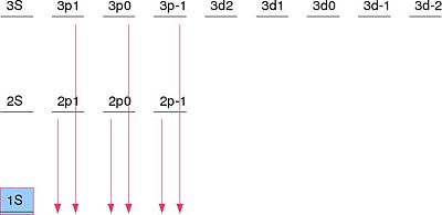
The possibles transitions to the state $2p_{0}$ are the following

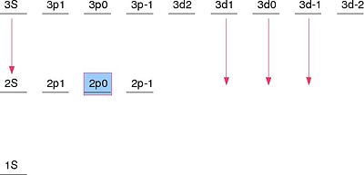
Power & Polarization of Emitted Light

Case $m'=m$: In this case the selection rules tells as that:

${\begin{aligned}\mathbf {d} _{0,n}=\langle 0|\mathbf {R} |n\rangle ={\begin{pmatrix}\langle 0|\mathbf {R} _{x}|n\rangle \\\langle 0|\mathbf {R} _{y}|n\rangle \\\langle 0|\mathbf {R} _{z}|n\rangle \\\end{pmatrix}}={\begin{pmatrix}0\\0\\\langle 0|\mathbf {R} _{z}|n\rangle \\\end{pmatrix}}\end{aligned}}$

Then we can say

• The light is always plane polarized in the plane defined by $\mathbf {k}$.
• The power is given by

  ${\begin{aligned}{\frac {dP}{d\Omega }}&\cong {\frac {e^{2}\omega _{n,0}^{4}}{2\pi c^{3}}}\left|\mathbf {d} _{0,n}\cdot \mathbf {\lambda } ^{*}\right|^{2}\\&\cong {\frac {e^{2}\omega _{n,0}^{4}}{2\pi c^{3}}}\left|\langle 0|\mathbf {R} _{z}|n\rangle \right|^{2}\;sin^{2}\theta \\\end{aligned}}$

Case $m'=m\pm 1$: In this case the selection rules tells as that:

${\begin{aligned}\mathbf {d} _{0,n}=\langle 0|\mathbf {R} |n\rangle ={\begin{pmatrix}\langle 0|\mathbf {R} _{x}|n\rangle \\\langle 0|\mathbf {R} _{y}|n\rangle \\\langle 0|\mathbf {R} _{z}|n\rangle \\\end{pmatrix}}={\begin{pmatrix}\langle 0|\mathbf {R} _{x}|n\rangle \\\langle 0|\mathbf {R} _{y}|n\rangle \\0\\\end{pmatrix}}\end{aligned}}$

From the previews result we have

${\begin{aligned}\mp \langle l'm'|\mathbf {R} _{y}|lm\rangle &=-i\langle l'm'|\mathbf {R} _{x}]lm\rangle \\\end{aligned}}$

Then

${\begin{aligned}\mathbf {d} _{0,n}=\langle 0|\mathbf {R} _{x}|n\rangle {\begin{pmatrix}1\\\pm i\\0\\\end{pmatrix}}\end{aligned}}$

Then we can say

• $\mathbf {d} _{0,n}$ rest at the XY plane. The polarization of the emitted light is circular.
• Lets put a detector to see the light coming toward positive Z axis. Since right circular polarized light has angular momentum $\hbar$ while negative circular polarized light has angular momentum$-\hbar$ we can state the following:
  • If we see a circular polarized light then by conservation of angular momentum we know that

    ${\begin{aligned}\hbar m=\hbar m'+\hbar ^{photon}\;\;\;\;\;\rightarrow \;\;\;\;\;m'-m=-1\end{aligned}}$

    the transition was $m'-m=-1$
  • If we see a negative circular polarized light then by conservation of angular momentum we know that

    ${\begin{aligned}\hbar m=\hbar m'-\hbar ^{photon}\;\;\;\;\;\rightarrow \;\;\;\;\;m'-m=1\end{aligned}}$

    the transition was $m'-m=1$

  Scattering of Light

  Non-perturbative methods

  One of the important method in the approximate determination of the wave function and eigenvalue is the Variational Principle. Variational method is a very general one that it can be used whenever the equations can be put into variational form.Variational principle is the springboard to many numerical computation.

  Principle of the Variational Method

  Consider a completely arbitrary system with time independent Hamiltonian ${\mathcal {H}}$ and we assume that it's entire spectrum is discrete and non-degenerate.

  ${\mathcal {H}}|{\varphi }_{n}\rangle$=${\mathcal {E}}_{n}|{\varphi }_{n}\rangle$ ; n = 0,1,2

  Let's apply the variational principle to find the ground state of the system.Let $|{\psi }\rangle$ be an arbitrary ket of the system. We can define the expectation value of the Hamiltonian as

  $\langle {\mathcal {H}}\rangle ={\frac {\langle {\psi }|{\mathcal {H}}|{\psi }\rangle }{\langle {\psi }|{\psi }\rangle }}\qquad {\text{(4.1)}}$

  The variational principle states that,

  $\langle {\mathcal {H}}\rangle \geq {\mathcal {E}}_{0}\qquad {\text{(4.2)}}$

  
  Since the exact eigenfunctions of $|{\varphi }\rangle$ form a complete set, we can express our arbitrary ket $|{\psi }\rangle$ as a linear combination of the exact wavefunction.Therefore,we have

  $|{\psi }\rangle =\sum _{n}C_{n}|{\varphi }_{n}\rangle \qquad {\text{(4.3)}}$

  Multiplying both sides by $\langle {\psi }|{\mathcal {H}}$ we get

  $\langle {\psi }|{\mathcal {H}}|{\psi }\rangle =\sum _{n}|C_{n}|^{2}\langle {\varphi }_{n}|{\varphi }_{n}\rangle =\sum _{n}|C_{n}|^{2}{\mathcal {E}}_{n}$

  
  However, ${\mathcal {E}}_{n}\geq {\mathcal {E}}_{0}$. So, we can write the above equation as

  $\langle {\psi }|{\mathcal {H}}|{\psi }\rangle \leq {\mathcal {E}}_{0}\sum _{n}|C_{n}|^{2}$

  Or

  ${\mathcal {E}}_{0}\leq {\frac {\langle {\psi }|{\mathcal {H}}|{\psi }\rangle }{\langle {\psi }|{\psi }\rangle }}\qquad {\text{(4.4)}}$.

  with ${\langle {\psi }|{\psi }\rangle }=\sum _{n}|C_{n}|^{2}$, thus proving $\qquad {\text{(4.2)}}$

  
  Thus $\qquad {\text{(4.2)}}$ gives an upper bound to the exact ground state energy. For the equality to be applicable in the $\qquad {\text{(4.2)}}$ all coefficients except ${\mathcal {C}}_{0}$ should be zero and then $|{\psi }\rangle$ will be the eigenvector of the Hamiltonian and ${\mathcal {E}}_{0}$ the ground state eigenvalue.

  
  

  Generalization of Variational Principle: The Ritz Theorem.

  We claim that the expectation value of the Hamiltonian is stationary in the neighborhood of its discrete eigenvalues. Let us again consider the expectation value of the Hamiltonian $\qquad {\text{(4.1)}}$

  $\langle {\mathcal {H}}\rangle ={\frac {\langle {\psi }|{\mathcal {H}}|{\psi }\rangle }{\langle {\psi }|{\psi }\rangle }}$

  Here $\langle {\mathcal {H}}\rangle$ is considered as a functional of $|\psi \rangle$. Let us define the variation of $\langle {\mathcal {H}}\rangle$ such that $|\psi \rangle$ goes to $|\psi \rangle +|\delta \psi \rangle$ where $|\delta \psi \rangle$ is considered to be infinetly small. Let us rewrite $\qquad {\text{(4.1)}}$ as

  $\langle {\mathcal {H}}\rangle \langle {\psi }|{\psi }\rangle =\langle {\psi }|{\mathcal {H}}|{\psi }\rangle \qquad {\text{(4.5)}}$.

  
  Differentiating the above relation,

  $\langle {\psi }|{\psi }\rangle \delta \langle {\mathcal {H}}\rangle +\langle {\mathcal {H}}\rangle [\langle {\psi }|\delta {\psi }\rangle +\langle \delta {\psi }|{\psi }\rangle ]=\langle {\psi }|{\mathcal {H}}|{\delta \psi }\rangle +\langle {\delta \psi }|{\mathcal {H}}|{\psi }\rangle \qquad {\text{(4.6)}}$

  
  However, $\langle {\mathcal {H}}\rangle$ is just a c-number, so we can rewrite $\qquad {\text{(4.6)}}$ as

  
  $\langle {\psi }|{\psi }\rangle \delta \langle {\mathcal {H}}\rangle =\langle {\psi }|[{\mathcal {H}}-\langle {\mathcal {H}}\rangle ]|{\delta \psi }\rangle +\langle {\delta \psi }|[{\mathcal {H}}-\langle {\mathcal {H}}\rangle ]|{\psi }\rangle \qquad {\text{(4.7)}}$.

  
  If $\delta |{\mathcal {H}}\rangle =0$, then the mean value of the Hamiltonian is stationary.

  Therefore,

  $\langle {\psi }|[{\mathcal {H}}-\langle {\mathcal {H}}\rangle ]|{\delta \psi }\rangle +\langle {\delta \psi }|[{\mathcal {H}}-\langle {\mathcal {H}}\rangle ]|{\psi }\rangle =0$.

  
  Define,

  $|{\varphi }\rangle =|[{\mathcal {H}}-\langle {\mathcal {H}}\rangle ]|{\psi }\rangle \qquad {\text{(4.8)}}$.

  Hence,$\qquad {\text{(4.7)}}$ become

  $\langle {\varphi }|\delta {\psi }\rangle +\langle \delta {\varphi }|{\psi }\rangle =0\qquad {\text{(4.9)}}$.

  
  We can define the variation of $|{\psi }\rangle$ as

  $|\delta {\psi }\rangle =\delta \lambda |\delta {\psi }\rangle$,

  
  with $\lambda$ being a small (real) number. Therefore $\qquad {\text{(4.9)}}$ can be written as

  $\langle {\psi }|{\psi }\rangle \delta \lambda =0\qquad {\text{(4.10)}}$

  Since the norm is zero, the wave function itself should be zero. Keeping this in mind, if we analyze $\qquad {(4.8)}$ it's clear that we can rewrite it as an eigenvalue problem.

  ${\mathcal {H}}|{\psi }\rangle =\langle {\mathcal {H}}\rangle {\psi }\rangle \qquad {\text{(4.11)}}$.

  
  Finally we can say that expectation value of the Hamiltonian is stationary iff the arbitrary wavefunction $|{\psi }\rangle$ is actually the eigenvector of the Hamiltonian with the stationary values of the expectation values of the Hamiltonian, $\langle {\mathcal {H}}\rangle$ being precisely the eigen values of the Hamiltonian.

  The general method is to find a approximate trial wavefunction that contain one or more parameters ${\mathcal {\alpha ,\beta ,\gamma }}$ . If the expectation value $\langle {\mathcal {H}}\rangle$ can be differentiated with respect to these paramters, the extrema of $\langle {\mathcal {H}}\rangle$ can be found using the following equation.

  ${\frac {\partial \langle {\mathcal {H}}\rangle }{\partial \alpha }}={\frac {\partial \langle {\mathcal {H}}\rangle }{\partial \beta }}={\frac {\partial \langle {\mathcal {H}}\rangle }{\partial \gamma }}=0$

  The absolute minimum of the expectation value of the Hamiltonian obtained by this method correspond to the upper bound on the ground state energy. The other relative, extrema corresponds to excited states.

  
  

  Upper Bound on First Excited State

  We claim that if $\langle {\psi }|{\varphi }_{0}\rangle =0$, then $\langle {\mathcal {H}}\rangle \geq {\mathcal {E}}_{1}$ where ${\mathcal {E}}_{1}$ is the energy of the first excited state and $|{\varphi }_{0}\rangle$ is the exact ground state of the Hamiltonian.

  From $\qquad {\text{(4.3)}}$ it is clear that if the above condition is satisfied then, ${\mathcal {C}}_{0}=0$. Therefore,we can write the expectation value of the hamiltonian as

  $\langle {\mathcal {H}}\rangle =\sum _{n=1}|{\mathcal {C}}_{n}|^{2}{\mathcal {E}}_{n}\geq {\mathcal {E}}_{1}\sum _{n=1}{\mathcal {|}}{C}_{n}|^{2}$

  Thus if we can find a suitable trial wavefunction that is orthogonal to the ground state exact wavefunction then by calculating the expectation value of the Hamiltonian, we get an upperbound on the first excited state. The trouble is that we might not know the exact ground state( which is one reason why we implement the variational principle). However if we have a Hamiltonian which is an even function, then the exact ground state will be an even function and hence any odd trial function will be a right candidate.

  
  

  Applications

  Harmonic Potential

  Armed with the variational method let us apply it first to a simple Hamiltonian. Consider the following Hamiltonian with harmonic potential whose eigenvalues and eigenfunctions are known exactly. We will determine how close we can get with a suitable trial function.

  
  ${\mathcal {H}}=-{\frac {\hbar ^{2}}{2m}}{\frac {d^{2}}{dx^{2}}}+{\frac {1}{2}}mw^{2}x^{2}\qquad \qquad {\text{(4.12)}}$

  
  The above hamiltonian is even therefore, to find the ground state upper bound we need to use an even trial function. Let us consider the following state vector with one parameter ${\mathcal {\alpha }}$

  
  $\psi (x)=Ae^{-\alpha x^{2}}:\alpha >0\qquad \qquad {\text{(4.13)}}$

  
  where $A\,\!$ is the normalization constant.

  
  

  Let us normalize the trial wavefunction to be unity

  $1=\langle \psi |\psi \rangle =|A|^{2}\int _{-\infty }^{\infty }e^{-2\alpha x^{2}}dx=|A|^{2}{\sqrt {\frac {\pi }{2\alpha }}}\Rightarrow A=\left[{\frac {2\alpha }{\pi }}\right]^{1/4}\qquad {\text{(4.14)}}$

  
  While, $\langle {\mathcal {H}}\rangle =|A|^{2}\int _{-\infty }^{\infty }dxe^{-\alpha x^{2}}\left[-{\frac {\hbar ^{2}}{2m}}{\frac {d^{2}}{dx^{2}}}+{\frac {1}{2}}mw^{2}x^{2}\right]e^{-\alpha x^{2}}={\frac {\hbar ^{2}\alpha }{2m}}+{\frac {mw^{2}}{8\alpha }}\qquad {\text{(4.15)}}$

  Minimizing the expectation value with respect to the parameter we get,

  ${\frac {d\langle {\mathcal {H}}\rangle }{d\alpha }}={\frac {\hbar ^{2}}{2m}}-{\frac {mw^{2}}{8\alpha ^{2}}}=0\Rightarrow \alpha ={\frac {mw}{2\hbar }}$

  
  Putting this value back in the expectation value we get

  $\langle {\mathcal {H}}\rangle _{min}={\frac {1}{2}}\hbar w$

  Due to our judicious selection of trial wavefunction, we were able to find the exact ground state energy. If we want to find the first excited state, a suitable candidate for trial wavefunction would be an odd function.

  A more general form involves an integer quantum number $n$:

  $\langle {\mathcal {H}}\rangle =\left(n+{\frac {1}{2}}\right)\hbar w$

  Ground State of Helium

  Let us use variational principle to determine the ground state energy of Helium. Helium has two electrons and two protons. For simplicity, we ignore the presence of neutrons.

  We can write the Hamiltonian can be written as

  
  $-{\frac {\hbar ^{2}}{2m}}({\boldsymbol {\nabla }}_{1}^{2}+{\boldsymbol {\nabla }}_{2}^{2})-{\frac {Ze^{2}}{|r_{1}|}}-{\frac {Ze^{2}}{|r_{2}|}}+{\frac {e^{2}}{|{\boldsymbol {r}}_{1}-{\boldsymbol {r}}_{2}|}}$

  
  where $\mathbf {r_{1},r_{2}}$ are the coordinates of the two electrons.

  If we ignore the mutual interaction term, then the wavefunction will be the product of the two individual electron wavefunction which in this case is that of a hydrogen like atom. Therefore,

  
  ${\mathcal {\psi }}({\boldsymbol {r_{1},r_{2}}})=\psi _{100}({\boldsymbol {r}}_{1})\psi _{100}({\boldsymbol {r}}_{2})\qquad {\text{(4.16)}}$

  where we ignored spin and

  $\psi _{100}=({\frac {Z^{3}}{\pi {a_{0}}^{3}}})^{1/2}exp(-{\frac {Zr}{a_{0}}})$

  
  Therefore we can write

  
  ${\mathcal {\psi }}_{100}{\boldsymbol {(r_{1},r_{2})}}={\frac {Z^{3}}{\pi {a_{0}}^{3}}}exp\left(-{\frac {Z(r_{1}+r_{2})}{a_{0}}}\right)\qquad {\text{(4.17)}}$

  
  We can write the ground state energy for this situation with $\mathbf {Z} =2$ as

  
  $E=2\left(-{\frac {m(2e^{2})^{2}}{2\hbar ^{2}}}\right)=-8Rd\simeq -108.8eV$

  However, the ground state energy has been experimentally determined accurately to -78.6 eV. Therefore our model is not a good one. Now let us apply variational method using a trial wavefunction. The trial wavefucntion we are going to is $\qquad {\text{(4.16)}}$ itself but with $\mathbf {Z}$ as variable. This argument is perfectly valid since each electron screens the nuclear charge seen by the other electron and hence the atomic number is less than 2.

  We can manipulate the Hamiltonian with ${\boldsymbol {Z}}$ going to $\mathbf {\sigma }$ and rewriting the potential term as ${\frac {\sigma e^{2}}{|r|}}+{\frac {(Z-\sigma )e^{2}}{|r|}}$. So the Hamiltonian becomes

  $H=-{\frac {\hbar ^{2}}{2m}}({\boldsymbol {\nabla }}_{1}^{2}+{\boldsymbol {\nabla }}_{2}^{2})-{\frac {\sigma e^{2}}{|r_{1}|}}+{\frac {(Z-\sigma )e^{2}}{|r_{1}|}}-{\frac {\sigma e^{2}}{|r_{2}|}}+{\frac {(Z-\sigma )e^{2}}{|r_{2}|}}+{\frac {e^{2}}{|{\boldsymbol {r}}_{1}-{\boldsymbol {r}}_{2}|}}$

  
  Now we can use the variational principle. The expectation value of the Hamiltonian is

  
  

  $\langle H\rangle =\int {d^{3}r_{1}}\int {d^{3}r_{2}}\psi *_{100}({\boldsymbol {r}}_{1})\psi *_{100}({\boldsymbol {r}}_{2})\left[-{\frac {\hbar ^{2}}{2m}}{\boldsymbol {\nabla }}_{1}^{2}-{\frac {\sigma e^{2}}{|r_{1}|}}+{\frac {(Z-\sigma )e^{2}}{|r_{1}|}}-{\frac {\hbar ^{2}}{2m}}{\boldsymbol {\nabla }}_{2}^{2}-{\frac {\sigma e^{2}}{|r_{2}|}}+{\frac {(Z-\sigma )e^{2}}{|r_{2}|}}+{\frac {e^{2}}{|{\boldsymbol {r}}_{1}-{\boldsymbol {r}}_{2}|}}\right]\psi _{100}({\boldsymbol {r}}_{1})\psi _{100}({\boldsymbol {r}}_{2})\qquad {\text{(4.18)}}$

  
  

  
  

  The first two terms give $E_{1}={\frac {-\sigma me^{4}}{2\hbar ^{2}}}$. The fourth and fifth term will give the same. The third term and sixth term nwill give

  $E_{2}=-{(Z-\sigma )e^{2}}\langle {\frac {1}{r_{1}}}\rangle =-{(Z-\sigma )e^{2}}{\frac {\sigma }{a_{0}}}$

  The seventh term will give an expectation value of

  
  $E_{3}={\frac {5\sigma me^{4}}{8\hbar ^{2}}}$

  
  Adding all this we get,

  $E=-{\frac {me^{4}}{2\hbar ^{2}}}\left(2\sigma ^{2}+4\sigma (Z-\sigma )-{\frac {5\sigma }{4}}\right)$

  
  

  Since $\mathbf {\sigma }$ is the variational parameter, we can minimize the Energy with respect to $\mathbf {\sigma }$. This will give us

  $\mathbf {\sigma } =Z-{\frac {5}{16}}$

  Putting $\mathbf {Z} =2$ we get $\mathbf {\sigma } =1.6875$ which is an improvemnet.

  
  Substituting this in $\qquad {\text{(4.16)}}$ we get $\mathbf {E} =-77.38eV$

  which is very close to the experimental value. Thus using variational principle we were able to calculate the ground state energy of the helium atom very close to the experimental value.

  Spin

  Spin 1/2 Angular Momentum

  The angular momentum of a stationary spin 1/2 particle is found to be quantized to the $\pm {\frac {\hbar }{2}}$ regardless of the direction of the axis chosen to measure the angular momentum. There is a vector operator ${\textbf {\overrightarrow {S}}}=(S_{x},S_{y},S_{z})$ when projected along an arbitrary axis satisfies the following equations:

  ${\overrightarrow {S}}\cdot {\hat {m}}|{\hat {m}}\uparrow \rangle ={\dfrac {\hbar }{2}}|{\hat {m}}\uparrow \rangle$

  ${\overrightarrow {S}}\cdot {\hat {m}}|{\hat {m}}\downarrow \rangle ={\dfrac {-\hbar }{2}}|{\hat {m}}\downarrow \rangle$

  $|{\hat {m}}\uparrow \rangle$ and $|{\hat {m}}\downarrow \rangle$ form a complete basis, which means that any state $|{\hat {n}}\uparrow \rangle$ and $|{\hat {n}}\downarrow \rangle$ can be expanded as a linear combination of $|{\hat {m}}\uparrow \rangle$ and $|{\hat {m}}\downarrow \rangle$.

  The spin operator obeys the standard angular momentum commutation relations

  $[S_{\mu },S_{\nu }]=i\hbar \epsilon _{\mu \nu \lambda }S_{\lambda }\Rightarrow [S_{x},S_{z}]=-i\hbar S_{y}$

  The most commonly used basis is the one which diagonalizes ${\overrightarrow {S}}\cdot {\hat {z}}=S_{z}$.

  By acting on the states $|{\hat {z}}\uparrow \rangle$ and $|{\hat {z}}\downarrow \rangle$ with ${\mathcal {S}}_{z}$, we find $S_{z}|{\hat {z}}\uparrow \rangle ={\dfrac {\hbar }{2}}|{\hat {z}}\uparrow \rangle$ $S_{z}|{\hat {z}}\downarrow \rangle ={\dfrac {-\hbar }{2}}|{\hat {z}}\downarrow \rangle$

  Now by acting to the left with another state, we can form a 2x2 matrix.

  ${\begin{aligned}S_{z}&=\left({\begin{array}{ll}\langle {\hat {z}}\uparrow |S_{z}|{\hat {z}}\uparrow \rangle &\langle {\hat {z}}\uparrow |S_{z}|{\hat {z}}\downarrow \rangle \\\langle {\hat {z}}\downarrow |S_{z}|{\hat {z}}\uparrow \rangle &\langle {\hat {z}}\downarrow |S_{z}|{\hat {z}}\downarrow \rangle \end{array}}\right)\\&=\left({\begin{array}{ll}\hbar /2&0\\0&-\hbar /2\end{array}}\right)\\&={\dfrac {\hbar }{2}}\left({\begin{array}{ll}1&0\\0&-1\end{array}}\right)\\&={\dfrac {\hbar }{2}}\sigma _{z}\end{aligned}}$

  where ${\mathcal {\sigma }}_{z}$ is the z Pauli spin matrix. Repeating the steps (or applying the commutation relations), we can solve for the x and y components.

  $S_{x}={\dfrac {\hbar }{2}}\left({\begin{array}{ll}0&1\\1&0\end{array}}\right)={\dfrac {\hbar }{2}}\sigma _{x}$

  
  $S_{y}={\dfrac {\hbar }{2}}\left({\begin{array}{ll}0&-i\\i&0\end{array}}\right)={\dfrac {\hbar }{2}}\sigma _{y}$

  
  It should be noted that a spin lying along an axis may be rotated to any other axis using the proper rotation operator.

  Properties of the Pauli Spin Matrices

  Each Pauli matrix squared produces the unity matrix

  $\sigma _{x}^{2}=\sigma _{y}^{2}=\sigma _{z}^{2}=\left({\begin{array}{ll}1&0\\0&1\end{array}}\right)$

  The commutation relation is as follows

  ${\mathcal {[\sigma _{\mu },\sigma _{\nu }]}}=2i\epsilon _{\mu \nu \lambda }\sigma _{\lambda }$

  and the anticommutator relation

  $\{\sigma _{\mu },\sigma _{\nu }\}=[\sigma _{\mu },\sigma _{\nu }]_{+}=\sigma _{\mu }\sigma _{\nu }+\sigma _{\nu }\sigma _{\mu }=2\delta _{\mu \nu }\left({\begin{array}{ll}0&1\\1&0\end{array}}\right)$

  For example, if ${\mathcal {\sigma _{\mu }\sigma _{\nu }=-\sigma _{\nu }\sigma _{\mu }}}$

  Then,

  $\sigma _{\mu }\sigma _{\nu }={\dfrac {1}{2}}[\sigma _{\mu },\sigma _{\nu }]+{\dfrac {1}{2}}{\sigma _{\mu },\sigma _{\nu }}=i\epsilon _{\mu \nu \lambda }\sigma _{\lambda }+\delta _{\mu \nu }$

  $S_{\mu }S_{\nu }={\dfrac {\hbar ^{2}}{4}}\delta _{\mu \nu }+{\dfrac {i\hbar }{2}}\epsilon _{\mu \nu \lambda }S_{\lambda }$

  The above equation is true for 1/2 spins only!!

  In general,

  ${\begin{aligned}(a\cdot \sigma )(b\cdot \sigma )&=(a_{x}\sigma _{x}+a_{y}\sigma _{y}+a_{z}\sigma _{z})(b_{x}\sigma _{x}+b_{y}\sigma _{y}+b_{z}\sigma _{z})\\&=a_{\mu }\sigma _{mu}b_{\nu }\sigma _{nu}\\&=a_{\mu }b_{\nu }\sigma _{mu}\sigma _{nu}\\&=a_{\mu }b_{\nu }\left(\left({\begin{array}{ll}1&0\\0&1\end{array}}\right)\delta _{\mu \nu }+i\epsilon _{\mu \nu \lambda }\sigma _{\lambda }\right)\\&=\left({\begin{array}{ll}1&0\\0&1\end{array}}\right)a\cdot b+i(a\times b)\cdot \sigma \end{aligned}}$

  Finally, any 2x2 matrix can be written in the form

  $M=\alpha \left({\begin{array}{ll}1&0\\0&1\end{array}}\right)+\beta \cdot \sigma =\left({\begin{array}{ll}M_{11}&M_{12}\\M_{21}&M_{22}\end{array}}\right)$

  $\Rightarrow \alpha ={\frac {1}{2}}(M_{11}+M_{22})$

  $\Rightarrow \beta _{x}={\frac {1}{2}}(M_{12}+M_{21})$

  $\Rightarrow \beta _{y}={\frac {i}{2}}(M_{12}-M_{21})$

  $\Rightarrow \beta _{z}={\frac {1}{2}}(M_{11}-M_{22})$

  for infinitesimal ${\mathcal {\alpha }}$

  

  ${\hat {n}}={\hat {m}}+{\overrightarrow {\alpha }}x{\hat {m}}+O(\alpha ^{2})$

  ${\overrightarrow {S}}\cdot {\hat {n}}={\overrightarrow {S}}\cdot {\hat {m}}+{\overrightarrow {S}}\cdot ({\overrightarrow {\alpha }}\times {\overrightarrow {m}})$

  $S_{\mu }{\hat {n_{\mu }}}=S_{\mu }{\hat {m_{\mu }}}+S_{\mu }\epsilon _{\mu \nu \lambda }\alpha _{\nu }{\hat {m_{\lambda }}}$

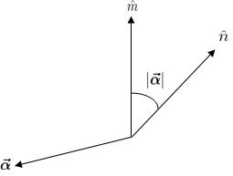
  Note that using the previous developed formulas, we find that

  ${\begin{aligned}S_{\mu }\epsilon _{\mu \nu \lambda }={\dfrac {1}{i\hbar }}[S_{\nu },S_{\lambda }]\Rightarrow {\overrightarrow {S}}\cdot {\hat {n}}&={\overrightarrow {S}}\cdot {\hat {m}}+{\dfrac {1}{i\hbar }}[{\overrightarrow {\alpha }}\cdot {\overrightarrow {S}},{\hat {m}}\cdot {\overrightarrow {S}}]\\&={\overrightarrow {S}}\cdot {\hat {m}}+{\dfrac {1}{i\hbar }}[{\overrightarrow {S}}\cdot {\hat {m}},{\overrightarrow {S}}\cdot {\overrightarrow {\alpha }}]\end{aligned}}$

  To this order in ${\overrightarrow {\alpha }}$:

  ${\overrightarrow {S}}\cdot {\hat {n}}=e^{-{\frac {i}{\hbar }}{\overrightarrow {S}}\cdot {\overrightarrow {\alpha }}}({\overrightarrow {S}}\cdot {\hat {m}})e^{{\frac {i}{\hbar }}{\overrightarrow {S}}\cdot {\overrightarrow {\alpha }}}$

  for finite $\alpha$ (correct for all orders)

  ${\overrightarrow {S}}\cdot {\hat {n}}\left(e^{-{\frac {i}{\hbar }}{\overrightarrow {S}}\cdot {\overrightarrow {\alpha }}}|{\hat {m}}\uparrow \rangle \right)={\dfrac {\hbar }{2}}\left(e^{-{\frac {i}{\hbar }}{\overrightarrow {S}}\cdot {\overrightarrow {\alpha }}}|{\hat {m}}\uparrow \rangle \right)$

  Addition of angular momenta

  Formalism

  Total angular momentum is defined as

  ${\overrightarrow {J}}={\overrightarrow {J_{1}}}+{\overrightarrow {J_{2}}}={\overrightarrow {J_{1}}}\otimes \left({\begin{array}{ll}1&0\\0&1\end{array}}\right)+\left({\begin{array}{ll}1&0\\0&1\end{array}}\right)\otimes {\overrightarrow {J_{2}}}\Rightarrow |j_{1}m_{1}\rangle \otimes |j_{2}m_{2}\rangle =|j_{1}j_{2}m_{1}m_{2}\rangle \qquad \qquad \qquad \qquad \qquad \qquad \qquad \quad (6.1.1)$

  where Hilbert space size is $\!(2j_{1}+1)(2j_{2}+1)$.

  We have the following commutation relations:

  $[J_{\mu },J_{\nu }]=i\hbar \epsilon _{\mu \nu \lambda }J_{\lambda }\qquad \qquad \qquad \qquad \qquad \qquad \qquad \qquad \qquad \qquad \qquad \qquad \qquad \qquad \qquad \qquad \qquad \qquad \qquad \qquad \;\ (6.1.2)$

  $[J_{1,2}^{2},J^{2}]=[J_{1,2}^{2},J_{z}]=0\qquad \qquad \qquad \qquad \qquad \qquad \qquad \qquad \qquad \qquad \qquad \qquad \qquad \qquad \qquad \qquad \qquad \qquad \qquad \;(6.1.3)$

  And consequently, $\![J^{2},J_{z}]=0\qquad \qquad \qquad \qquad \qquad \qquad \qquad \qquad \qquad \qquad \qquad \qquad \qquad \qquad \qquad \qquad \qquad \qquad \qquad \qquad \qquad \quad (6.1.4)$

  However, $[J^{2},J_{1z,2z}]\neq 0$. Therefore, to construct a basis, one can not take a direct product between the set of eigenkets of $\!J^{2}$ and those of $\!J_{1z,2z}$. For example,
  assume two spin 1/2 particles with basis ${|\uparrow \uparrow \rangle ,|\uparrow \downarrow \rangle ,|\downarrow \uparrow \rangle ,|\downarrow \downarrow \rangle }$. These states are eigenstates of $J_{1}^{2},J_{2}^{2},J_{1z},J_{2z}$, but are they eigenstates of $\!J^{2}$ and $J_{z}^{2}$?
  Let us see what happens with the state $|\uparrow \downarrow \rangle$:

  $J^{2}|\uparrow \downarrow \rangle =(J_{x}^{2}+J_{y}^{2}+J_{z}^{2})|\uparrow \downarrow \rangle =((J_{x}+iJ_{y})(J_{x}-iJ_{y})+i[J_{x},J_{y}]+J_{z}^{2})|\uparrow \downarrow \rangle$

  define $J_{\pm }=(J_{x}\pm iJ_{y})$

  $J^{2}|\uparrow \downarrow \rangle =(J_{+}J_{-}-\hbar J_{z}+J_{z}^{2})|\uparrow \downarrow \rangle =((J_{1+}+J_{2+})(J_{1-}+J_{2-})+(J_{1z}+J_{2z})^{2}-\hbar (J_{1z}+J_{2z}))|\uparrow \downarrow \rangle$

  Now $(J_{1z}+J_{2z})|\uparrow \downarrow \rangle =({\dfrac {\hbar }{2}}-{\dfrac {\hbar }{2}})|\uparrow \downarrow \rangle =0$

  Also, $(J_{1+}+J_{2+})(J_{1-}+J_{2-})|\uparrow \downarrow \rangle =(J_{1+}+J_{2+})|\downarrow \downarrow \rangle =|\uparrow \downarrow \rangle +|\downarrow \uparrow \rangle$

  $\therefore J^{2}|\uparrow \downarrow \rangle =|\uparrow \downarrow \rangle +|\downarrow \uparrow \rangle$

  Which means that $|\uparrow \downarrow \rangle$ is not an eigenstate of $\!J^{2}$. Similarly, it can be shown that the other three states are also not eigenstates of $\!J^{2}$. As a result, there are two
  choices for sets of base kets which can be used:

  1. The simultaneous eigenkets of $J_{1}^{2}$, $J_{2}^{2}$, $\!J_{1z}$, $\!J_{2z}$, denoted by $|j_{1}j_{2}m_{1}m_{2}\rangle$. These four operators commute with each other, and they operate on the base kets
  according to:

  $J_{1,2}^{2}|j_{1}j_{2}m_{1}m_{2}\rangle =\hbar _{2}j_{1,2}(j_{1,2}+1)|j_{1}j_{2}m_{1}m_{2}\rangle \qquad \qquad \qquad \qquad \qquad \qquad \qquad \qquad \qquad \qquad \qquad \qquad \qquad \qquad \qquad \;(6.1.5)$

  $J_{1z,2z}|j_{1}j_{2}m_{1}m_{2}\rangle =\hbar m_{1,2}|j_{1}j_{2}m_{1}m_{2}\rangle \qquad \qquad \qquad \qquad \qquad \qquad \qquad \qquad \qquad \qquad \qquad \qquad \qquad \qquad \qquad \qquad \quad (6.1.6)$

  2. The simultaneous eigenkets of $\!J^{2}$, $J_{1}^{2}$, $J_{2}^{2}$ and $J_{z}$, denoted by $|jmj_{1}j_{2}\rangle$. These four operators operate on the base kets according to:

  $J^{2}|jmj_{1}j_{2}\rangle =\hbar ^{2}j(j+1)|jmj_{1}j_{2}\rangle \qquad \qquad \qquad \qquad \qquad \qquad \qquad \qquad \qquad \qquad \qquad \qquad \qquad \qquad \qquad \qquad \qquad \;\;\;\;(6.1.7)$

  $J_{z}|jmj_{1}j_{2}\rangle =\hbar m|jmj_{1}j_{2}\rangle \qquad \qquad \qquad \qquad \qquad \qquad \qquad \qquad \qquad \qquad \qquad \qquad \qquad \qquad \quad \;\;\;\;\;\ (6.1.8)$

  $J_{1,2}^{2}|jmj_{1}j_{2}\rangle =\hbar ^{2}j_{1,2}(j_{1,2}+1)|jmj_{1}j_{2}\rangle \qquad \qquad \qquad \qquad \qquad \qquad \qquad \qquad \qquad \qquad \qquad \qquad \quad \;\;\ (6.1.9)$

  
  

  Clebsch-Gordan Coefficients

  Now that we have constructed two different bases of eigenkets, it is imperative to devise a way such that eigenkets of one basis may be written as

  linear combinations of the eigenkets of the other basis. To achieve this, we write:

  $|jmj_{1}j_{2}\rangle =\sum _{m_{1},m_{2}}|j_{1}j_{2}m_{1}m_{2}\rangle \langle j_{1}j_{2}m_{1}m_{2}|jmj_{1}j_{2}\rangle \qquad \qquad \qquad \qquad \qquad \qquad \qquad \qquad \qquad \qquad \quad \ (6.2.1)$

  In above, we have used the completeness of the basis $|j_{1}j_{2}m_{1}m_{2}\rangle$, given by:

  $\sum _{m_{1},m_{2}}|j_{1}j_{2}m_{1}m_{2}\rangle \langle j_{1}j_{2}m_{1}m_{2}|=1\qquad \qquad \qquad \qquad \qquad \qquad \qquad \qquad \qquad \qquad \qquad \qquad \qquad \quad \;\;\;(6.2.2)$

  The coefficients $\langle j_{1}j_{2}m_{1}m_{2}|jmj_{1}j_{2}\rangle$ are called Clebsch-Gordan coefficients, which have the following properties, giving rise to two
  "selection rules":

  1. If $m\neq m_{1}+m_{2}$, then the coefficients vanish.

  Proof: $\because J_{z}=J_{1z}+J_{2z}$, we get

  $(J_{z}-J_{1z}-J_{2z})|jmj_{1}j_{2}\rangle =0$

  $\Rightarrow \langle j_{1}j_{2}m_{1}m_{2}|(J_{z}-J_{1z}-J_{2z})|jmj_{1}j_{2}\rangle =0$

  $\therefore (m-m_{1}-m_{2})\langle j_{1}j_{2}m_{1}m_{2}|jmj_{1}j_{2}\rangle =0$. Q.E.D.

  2. The coefficients vanish, unless $|j_{1}-j_{2}|\leq j\leq j_{1}+j_{2}$

  This follows from a simple counting argument. Let us assume, without any loss of generality, that $\!j_{1}>j_{2}$. The dimensions of the two bases should

  be the same. If we count the dimensions using the $|j_{1}j_{2}m_{1}m_{2}\rangle$ states, we observe that for any value of $\!j$, the values of $\!m$ run from $\!-j$ to $\!j$.

  Therefore, for $\!j_{1}$ and $\!j_{2}$, the number of eigenkets is $\!(2j_{1}+1)(2j_{2}+1)$. Now, counting the dimensions using the $|jmj_{1}j_{2}\rangle$ eigenkets, we

  observe that, again, $\!m$ runs from $\!-j$ to $\!j$. Therefore, the number of dimensions is $N=\sum _{a}^{b}(2j+1)$. It is easy to see that for

  $\!a=j_{1}-j_{2}$ and $\!b=j_{1}+j_{2},N=(2j_{1}+1)(2j_{2}+1)$.

  Further, it turns out that, for fixed $\!j_{1}$, $\!j_{2}$ and $\!j$, coefficients with different values for $\!m_{1}$ and $\!m_{2}$ are related to each other through recursion

  relations. To derive these relations, we first note that: $J_{\pm }|jmj_{1}j_{2}\rangle ={\sqrt {(j\mp m)(j\pm m+1)}}\hbar |jm\pm 1j_{1}j_{2}\rangle \qquad \qquad \qquad \qquad \qquad \qquad \qquad \qquad \qquad \qquad \;\ (6.2.3)$

  Now we write, $J_{\pm }|jmj_{1}j_{2}\rangle =(J_{1\pm }+J_{2\pm })\sum _{m_{1},m_{2}}|j_{1}j_{2}m_{1}m_{2}\rangle \langle j_{1}j_{2}m_{1}m_{2}|jmj_{1}j_{2}\rangle \qquad \qquad \qquad \qquad (6.2.4)$

  Using equation #(6.2.4), we get (with $m_{1}\to m'_{1}$, $m_{2}\to m'_{2}$):
  ${\begin{aligned}{\sqrt {(j\mp m)(j\pm m+1)}}|jm\pm 1j_{1}j_{2}\rangle =\sum _{m'_{1},m'_{2}}({\sqrt {(j_{1}\mp m'_{1})(j_{1}\pm m'_{1}+1)}}|j_{1}j_{2}m'_{1}\pm 1m'_{2}\rangle \ +\\{\sqrt {(j_{2}\mp m'_{2})(j_{2}\pm m'_{2}+1)}}|j_{1}j_{2}m'_{1}m'_{2}\pm 1\rangle )\langle j_{1}j_{2}m'_{1}m'_{2}|jmj_{1}j_{2}\rangle \end{aligned}}$

  
  The Clebsch-Gordan coefficients form a unitary matrix, and by convention, they are all taken real. Any real unitary matrix is orthogonal, as we study

  below.

  
  

  Orthogonality of Clebsch-Gordan Coefficients

  Using the additon of angular momentum, $|j_{1}m_{1}j_{2}m_{2}\rangle$ where there are $\!(2j_{1}+1)(2j_{2}+1)$ states, one can get $|jmj_{1}j_{2}\rangle$ where $\!j=|j_{1}-j_{2}|,...,j_{1}+j_{2}$, the last of which is an eigenvector for $\!J^{2},J_{z},$ etc.

  $|jmj_{1}j_{2}\rangle =\sum _{m_{1},m_{2}}|j_{1}m_{1}j_{2}m_{2}\rangle \langle j_{1}m_{1}j_{2}m_{2}|jmj_{1}j_{2}\rangle$

  where $\langle j_{1}m_{1}j_{2}m_{2}|jmj_{1}j_{2}\rangle$ are the Clebsch-Gordon Coefficients. CG's are real and the following is convention:

  $\langle j_{1}j_{1}j_{2}j-j_{1}|jjj_{1}j_{2}\rangle$ is positive and there is the following symmetry:

  $\langle j_{1}m_{1}j_{2}m_{2}|jmj_{1}j_{2}\rangle =(-1)^{j_{1}+j_{2}-j}\langle j_{1},-m_{1},j_{2},-m_{2}|j,-m,j_{1},j_{2}\rangle$

  If we put the coefficients into a matrix, it is real and unitary, meaning $\langle jmj_{1}j_{2}|j_{1}m_{1}j_{2}m_{2}\rangle =\langle j_{1}m_{1}j_{2}m_{2}|jmj_{1}j_{2}\rangle ^{*}$

  $|j_{1}m_{1}j_{2}m_{2}\rangle =\sum _{j,m}|jmj_{1}j_{2}\rangle \langle jmj_{1}j_{2}|j_{1}m_{1}j_{2}m_{2}\rangle$

  $|\uparrow _{1}\downarrow _{2}\rangle ={\dfrac {1}{\sqrt {2}}}(|10\rangle +|00\rangle )$

  $|\downarrow _{1}\uparrow _{2}\rangle ={\dfrac {1}{\sqrt {2}}}(|10\rangle -|00\rangle )$

  $\sum _{jm}\langle j_{1}m'_{1}j_{2}m'_{2}|jmj_{1}j_{2}\rangle \langle jmj_{1}j_{2}|j_{1}m_{1}j_{2}m_{2}\rangle =\delta _{m_{1}m'_{1}}\delta _{m_{2}m'_{2}}$

  $\sum _{m_{1}m_{2}}\langle jmj_{1}j_{2}|j_{1}m_{1}j_{2}m_{2}\rangle \langle j_{1}m_{1}j_{2}m_{2}|j'm'j_{1}j_{2}\rangle =\delta _{jj'}\delta _{mm'}$

  Hydrogen atom with spin orbit coupling given by the following hamiltonian

  $H'={\dfrac {c^{2}}{2m^{2}c^{2}r^{3}}}{\overrightarrow {L}}\cdot {\overrightarrow {S}}$

  Recall, the atomic spectrum for bound states

  $E_{n}={\dfrac {-e^{2}}{2a_{o}}}{\dfrac {1}{n^{2}}}$ $;n=1,2,3,...$

  The ground state, $|1s\rangle$, is doubly degenerate: ${\dfrac {\uparrow \downarrow }{1s}}$

  First excited state is 8-fold degenerate: ${\dfrac {\uparrow \downarrow }{1s}}{\dfrac {\uparrow \downarrow }{}}{\dfrac {\uparrow \downarrow }{2p}}{\dfrac {\uparrow \downarrow }{}}$

  nth state is $2n^{2}$ fold degenerate

  We can break apart the angular momentum and spin into its x, y, z-components

  ${\overrightarrow {L}}\cdot {\overrightarrow {S}}=L_{x}S_{x}+L_{y}S_{y}+L_{z}S_{z}$

  Define lowering and raising operators

  $\Rightarrow L_{\pm }=L_{x}\pm iL_{y}$

  $\Rightarrow S_{\pm }=S_{x}\pm iS_{y}$

  ${\overrightarrow {L}}\cdot {\overrightarrow {S}}=L_{z}S_{z}+{\dfrac {1}{2}}L_{+}S_{-}+{\dfrac {1}{2}}L_{-}S_{+}$

  For the ground state, $(|1s,\uparrow \rangle ,|1s,\downarrow \rangle )$, nothing happens. Kramer's theorem protects the double degeneracy.

  For the first excited state, $(|2s,\uparrow \rangle ,|2s,\downarrow \rangle )$, once again nothing happens.

  For $(|2p,\uparrow \rangle ,|2p,\downarrow \rangle )$, there is a four fold degeneracy.

  We can express the solutions in matrix form

  $\left({\begin{array}{llllll}{\dfrac {\hbar ^{2}}{2}}&0&0&0&0&0\\0&0&0&0&0&0\\0&0&0&0&0&0\\0&0&0&0&0&0\\0&0&0&0&0&0\\0&0&0&0&0&{\dfrac {\hbar ^{2}}{2}}\end{array}}\right)$

  But there is a better and more exact solution, which we can solve for by adding the momenta first.

  ${\overrightarrow {L}}\cdot {\overrightarrow {S}}={\dfrac {1}{2}}({\overrightarrow {L}}+{\overrightarrow {S}})^{2}-{\dfrac {1}{2}}{\overrightarrow {L^{2}}}-{\dfrac {1}{2}}{\overrightarrow {S^{2}}}={\dfrac {1}{2}}(J^{2}-L^{2}-S^{2})$

  add the angular momenta:

  $|1s\rangle :l=0,s={\dfrac {1}{2}}:0\otimes {\dfrac {1}{2}}={\dfrac {1}{2}}$

  $|2s\rangle :l=0,s={\dfrac {1}{2}}:0\otimes {\dfrac {1}{2}}={\dfrac {1}{2}}$

  $|2p_{m},0\rangle :l=1,s={\dfrac {1}{2}}:1\otimes {\dfrac {1}{2}}={\dfrac {3}{2}}\oplus {\dfrac {1}{2}}$

  So that

  ${\overrightarrow {L}}\cdot {\overrightarrow {S}}|j={\dfrac {3}{2}},m,l=1,s={\dfrac {1}{2}}\rangle ={\dfrac {1}{2}}(\hbar ^{2}{\dfrac {3}{2}}{\dfrac {5}{2}}-2\hbar ^{2}-{\dfrac {3}{4}}\hbar ^{2})|j={\dfrac {3}{2}},m,l=1,s={\dfrac {1}{2}}\rangle ={\dfrac {\hbar ^{2}}{2}}|j={\dfrac {3}{2}},m,l=1,s={\dfrac {1}{2}}\rangle$

  ${\overrightarrow {L}}\cdot {\overrightarrow {S}}|j={\dfrac {1}{2}},m,l=1,s={\dfrac {1}{2}}\rangle ={\dfrac {-\hbar ^{2}}{2}}|j={\dfrac {1}{2}},m,l=1,s={\dfrac {1}{2}}\rangle$

  $|j={\dfrac {3}{2}},m={\dfrac {3}{2}},l=1,s={\dfrac {1}{2}}\rangle =|l=1,m_{l}=1\rangle |s={\dfrac {1}{2}},m_{s}={\dfrac {1}{2}}\rangle$

  $|j={\dfrac {3}{2}},m={\dfrac {3}{2}}\rangle =|m_{l}=1\rangle |m_{s}={\dfrac {1}{2}}\rangle$

  Define J_

  $J_{|}{\dfrac {3}{2}},{\dfrac {1}{2}}\rangle =(L_{+}S_{)}|1\rangle |{\dfrac {1}{2}}\rangle$

  
  $\hbar {\sqrt {{\dfrac {3}{2}}{\dfrac {5}{2}}-{\dfrac {3}{2}}{\dfrac {1}{2}}}}|{\dfrac {3}{2}},{\dfrac {1}{2}}\rangle =\hbar {\sqrt {2}}|0\rangle |{\dfrac {1}{2}}\rangle +\hbar {\sqrt {{\dfrac {1}{2}}{\dfrac {3}{2}}+{\dfrac {1}{4}}}}|1,-{\dfrac {1}{2}}\rangle$

  
  ${\sqrt {3}}|{\dfrac {3}{2}},{\dfrac {1}{2}}\rangle ={\sqrt {2}}|0\rangle |{\dfrac {1}{2}}\rangle +|1,-{\dfrac {1}{2}}\rangle$

  $|{\dfrac {3}{2}},{\dfrac {1}{2}}\rangle ={\sqrt {\dfrac {2}{3}}}|0\rangle |{\dfrac {1}{2}}\rangle +{\sqrt {\dfrac {1}{3}}}|1\rangle |-{\dfrac {1}{2}}\rangle$

  $|{\dfrac {3}{2}},{\dfrac {-1}{2}}\rangle ={\sqrt {\dfrac {2}{3}}}|0\rangle |{\dfrac {-1}{2}}\rangle +{\sqrt {\dfrac {1}{3}}}|-1\rangle |{\dfrac {1}{2}}\rangle$

  $|{\dfrac {3}{2}},{\dfrac {-3}{2}}\rangle =|-1\rangle |-{\dfrac {1}{2}}\rangle$

  Can express as

  $|j={\dfrac {1}{2}},m={\dfrac {1}{2}}\rangle =\alpha |0\rangle |{\dfrac {1}{2}}\rangle +\beta |1\rangle |-{\dfrac {1}{2}}\rangle$

  $|j={\dfrac {1}{2}},m=-{\dfrac {1}{2}}\rangle =\alpha '|0\rangle |-{\dfrac {1}{2}}\rangle +\beta '|-1\rangle |{\dfrac {1}{2}}\rangle$

  When we project these states on the previously found states $\left(\langle {\dfrac {3}{2}}{\dfrac {1}{2}}|{\dfrac {1}{2}}{\dfrac {1}{2}}\rangle =0\right)$ we find that

  $\alpha =-{\dfrac {1}{\sqrt {3}}}$ and $\beta ={\sqrt {\dfrac {2}{3}}}$

  Elementary applications of group theory in Quantum Mechanics

  Irreducible tensor representations and Wigner-Eckart theorem

  Elements of relativistic quantum mechanics

  In nonrelativistic quantum mechanics, states of particles are described by Schrodinger equation of states:

  $i\hbar {\frac {\partial \psi ({\mathbf {r}},t)}{\partial t}}=(-{\frac {\hbar ^{2}}{2m}}\nabla ^{2}+V({\mathbf {r}},t))\psi ({\mathbf {r}},t)$

  Schrodinger equation is a first order in time. However, it is a second order in space. Therefore, it is not invariant under the Lorentz transformation. Equation of states in relativistic quantum mechanics must be invariant under the Lorentz transformation. In order to satisfy this condition, equation of state must contain the derivatives with respect to time and space of the same order. Equations of states in relativistic quantum mechanics are Klein-Gordon equation (for spinless particles) and Dirac equation (for spin ${\frac {1}{2}}$ particles). The former contains second ordered derivatives while the latter contains first ordered derivatives with respect to both time and space. The way to derive these equations is similar to that of Schrodinger equation: starting from the equation connecting energy and momentum, substituting $E$ by $i\hbar {\frac {\partial }{\partial t}}$ and ${\mathbf {p}}$ by $-i\hbar \nabla$.

  Follow this link to learn about Klein-Gordon equation.

  Follow this link to learn about Dirac equation.