PHY6937

Welcome to Phy 6937 Superconductivity and superfluidity

PHY6937 is a one semester advanced graduate level course. Its aim is to introduce concepts and theoretical techniques for the description of superconductors and superfluids. This course is a natural continuation of the "many-body" course PHY5670 and will build on the logical framework introduced therein, i.e. broken symmetry and adiabatic continuity. The course will cover a range of topics, such as the connection between the phenomenological Ginzburg-Landau and the microscpic BCS theory, Migdal-Eliashberg treatment of phonon mediated superconductivity, unconventional superconductivity, superfluidity in He-4 and He-3, and Kosterlitz-Thouless theory of two dimensional superfluids.

The key component of the course is the collaborative student contribution to the course Wiki-textbook. Each team of students is responsible for BOTH writing the assigned chapter AND editing chapters of others.

Team assignments: Spring 2011 student teams

---

Outline of the course:

Pairing Hamiltonian and BCS instability

To see the origins of superconductivity, it is helpful to look at a toy system, which we already know will give us superconducting behavior. This is useful because the toy system is only a simple change to a non-interacting electron gas. By adding in some small attractive interaction, we will arrive at a superconducting system! This interaction need only occur between two electrons occupying the same position in space (and necessarily having opposite spin!). Additionally, we still find the interesting behaviour regardless of the size of the interaction; the only requirement is that it be non-zero!

We can write the Hamiltonian of the system as:

Failed to parse (SVG (MathML can be enabled via browser plugin): Invalid response ("Math extension cannot connect to Restbase.") from server "https://wikimedia.org/api/rest_v1/":): {\displaystyle H=\sum_\vec{r}[\psi_\sigma^\dagger (\vec{r})(\epsilon_\vec{p}-\mu)\psi_\sigma^\dagger (\vec{r}) +g\psi_\uparrow^\dagger (\vec{r})\psi_\downarrow^\dagger (\vec{r})\psi_\downarrow (\vec{r})\psi_\uparrow (\vec{r})]}

where Failed to parse (SVG (MathML can be enabled via browser plugin): Invalid response ("Math extension cannot connect to Restbase.") from server "https://wikimedia.org/api/rest_v1/":): {\displaystyle \ g<0} and Failed to parse (SVG (MathML can be enabled via browser plugin): Invalid response ("Math extension cannot connect to Restbase.") from server "https://wikimedia.org/api/rest_v1/":): {\displaystyle \ |g|<<\epsilon_{F}} .

For this system, the partition function is:

Failed to parse (SVG (MathML can be enabled via browser plugin): Invalid response ("Math extension cannot connect to Restbase.") from server "https://wikimedia.org/api/rest_v1/":): {\displaystyle Z=\int D[\psi_\sigma ^{*} (\tau, \vec{r}), \psi_\sigma (\tau, \vec{r})]e^{-S_{BCS}}}

where Failed to parse (SVG (MathML can be enabled via browser plugin): Invalid response ("Math extension cannot connect to Restbase.") from server "https://wikimedia.org/api/rest_v1/":): {\displaystyle S_{BCS}=\int_0^\beta d\tau \sum_\vec{r}[\psi_\sigma^\dagger (\tau, \vec{r})(\partial _\tau+\epsilon_\vec{p}-\mu)\psi_\sigma^\dagger (\vec{r}) +g\psi_\uparrow^\dagger (\vec{r})\psi_\downarrow^\dagger (\vec{r})\psi_\downarrow (\vec{r})\psi_\uparrow (\vec{r})]}

It doesn't matter to multiply partition function by a constant:

Failed to parse (SVG (MathML can be enabled via browser plugin): Invalid response ("Math extension cannot connect to Restbase.") from server "https://wikimedia.org/api/rest_v1/":): {\displaystyle Z\rightarrow Z=\int D[\psi_\sigma ^{*} (\tau, \vec{r}), \psi_\sigma (\tau, \vec{r})] D[\Delta^{*}(\tau, \vec{r}),\Delta (\tau, \vec{r})] e^{-S_{BCS}-S_{\Delta}}}

where Failed to parse (SVG (MathML can be enabled via browser plugin): Invalid response ("Math extension cannot connect to Restbase.") from server "https://wikimedia.org/api/rest_v1/":): {\displaystyle S_\Delta=-\int_0^\beta d\tau\sum_{\vec{r}}\frac{1}{g}\Delta^*(\tau,\vec{r})\Delta(\tau,\vec{r})}

Failed to parse (SVG (MathML can be enabled via browser plugin): Invalid response ("Math extension cannot connect to Restbase.") from server "https://wikimedia.org/api/rest_v1/":): {\displaystyle \psi^\dagger} and Failed to parse (SVG (MathML can be enabled via browser plugin): Invalid response ("Math extension cannot connect to Restbase.") from server "https://wikimedia.org/api/rest_v1/":): {\displaystyle \ \psi} are grassmann numbers. Failed to parse (SVG (MathML can be enabled via browser plugin): Invalid response ("Math extension cannot connect to Restbase.") from server "https://wikimedia.org/api/rest_v1/":): {\displaystyle \ \Delta^*} and Failed to parse (SVG (MathML can be enabled via browser plugin): Invalid response ("Math extension cannot connect to Restbase.") from server "https://wikimedia.org/api/rest_v1/":): {\displaystyle \ \Delta} are constant. Failed to parse (SVG (MathML can be enabled via browser plugin): Invalid response ("Math extension cannot connect to Restbase.") from server "https://wikimedia.org/api/rest_v1/":): {\displaystyle \psi_\uparrow\psi_\downarrow} and Failed to parse (SVG (MathML can be enabled via browser plugin): Invalid response ("Math extension cannot connect to Restbase.") from server "https://wikimedia.org/api/rest_v1/":): {\displaystyle \psi_\downarrow\psi_\uparrow} behave like constant.

Let's make a shift of the constant:

Failed to parse (SVG (MathML can be enabled via browser plugin): Invalid response ("Math extension cannot connect to Restbase.") from server "https://wikimedia.org/api/rest_v1/":): {\displaystyle \Delta \rightarrow \Delta+g\psi_\uparrow\psi_\downarrow}

Failed to parse (SVG (MathML can be enabled via browser plugin): Invalid response ("Math extension cannot connect to Restbase.") from server "https://wikimedia.org/api/rest_v1/":): {\displaystyle \Delta^*\rightarrow \Delta^*+g\psi^\dagger_\downarrow\psi^\dagger_\uparrow}

Then, Failed to parse (SVG (MathML can be enabled via browser plugin): Invalid response ("Math extension cannot connect to Restbase.") from server "https://wikimedia.org/api/rest_v1/":): {\displaystyle S_\Delta=-\int_0^\beta d\tau \sum_{\vec{r}}{\{\frac{1}{g}\Delta^*\Delta + \Delta^*\psi_\uparrow \psi_\downarrow + \Delta\psi^\dagger_\downarrow \psi^\dagger_\uparrow+g\psi^\dagger_\downarrow \psi^\dagger_\uparrow \psi_\uparrow \psi_\downarrow}\}}

Failed to parse (SVG (MathML can be enabled via browser plugin): Invalid response ("Math extension cannot connect to Restbase.") from server "https://wikimedia.org/api/rest_v1/":): {\displaystyle \begin{align}S=&S_{BCS}+S_{\Delta}\\ =&\int_0^\beta d\tau \sum_{\vec{r}}\{ \psi_\sigma^\dagger(\tau, \vec{r})(\partial _\tau+\epsilon_\vec{p}-\mu)\psi_\sigma^\dagger (\tau, \vec{r}) \ \ \ \ \ \ \ \ \ \ \rightarrow S_0 \\ &+\Delta^*(\tau, \vec{r})\psi_\uparrow (\tau, \vec{r})\psi_\downarrow (\tau, \vec{r}) \Delta (\tau, \vec{r})\psi^\dagger_\downarrow (\tau, \vec{r})\psi^\dagger_\uparrow (\tau, \vec{r}) \rightarrow S_{int}\\ &-\frac{1}{g}\Delta^* (\tau, \vec{r})\Delta (\tau, \vec{r}) \} \ \ \ \ \ \ \ \ \ \ \ \ \ \ \ \ \ \ \ \ \ \ \ \ \ \ \ \ \ \ \ \ \ \ \ \rightarrow S_{\Delta} \end{align}}

then, Failed to parse (SVG (MathML can be enabled via browser plugin): Invalid response ("Math extension cannot connect to Restbase.") from server "https://wikimedia.org/api/rest_v1/":): {\displaystyle Z=\int D[\psi_{\sigma}^{*}(\tau,\mathbf{r}),\psi_{\sigma}(\tau,\mathbf{r})]D[\Delta^{*}(\tau,\mathbf{r}),\Delta(\tau,\mathbf{r})]e^{-(S_{0}+S_{int.}+S_{\Delta})}} .

Failed to parse (SVG (MathML can be enabled via browser plugin): Invalid response ("Math extension cannot connect to Restbase.") from server "https://wikimedia.org/api/rest_v1/":): {\displaystyle \left\langle e^{-S_{int.}}\right\rangle _{0}\cong exp[\frac{1}{2}\left\langle S_{int.}^{2}\right\rangle _{0}+\frac{1}{4!}(\left\langle S_{int.}^{4}\right\rangle _{0}-3\left\langle S_{int.}^{2}\right\rangle _{0}^{2})]} by cumulant expansion, which guarantees that until the 2nd order, it is accurate.

Use Matsubara's Method

Failed to parse (SVG (MathML can be enabled via browser plugin): Invalid response ("Math extension cannot connect to Restbase.") from server "https://wikimedia.org/api/rest_v1/":): {\displaystyle \psi_{\sigma}(\tau,\mathbf{r})=\frac{1}{\beta}\underset{\omega_{n}}{\sum}\underset{\mathbf{k}}{\sum}e^{i\mathbf{k}\cdot\mathbf{r}}e^{-i\omega_{n}\tau}\psi_{\sigma}(i\omega_{n},\mathbf{k}), \omega_{n}=(2n+1)\frac{\pi}{\beta};}

Failed to parse (SVG (MathML can be enabled via browser plugin): Invalid response ("Math extension cannot connect to Restbase.") from server "https://wikimedia.org/api/rest_v1/":): {\displaystyle \Delta(\tau,\mathbf{r})=\frac{1}{\beta}\underset{\Omega_{n}}{\sum}\underset{\mathbf{k}}{\sum}e^{i\mathbf{k}\cdot\mathbf{r}}e^{-i\Omega_{n}\tau}\Delta_{\mathbf{k}}(i\Omega_{n}), \omega_{n}=2n\frac{\pi}{\beta}.}

Then Failed to parse (SVG (MathML can be enabled via browser plugin): Invalid response ("Math extension cannot connect to Restbase.") from server "https://wikimedia.org/api/rest_v1/":): {\displaystyle S_{0}=\frac{L^{D}}{\beta}\underset{\omega_{n}}{\sum}\underset{\mathbf{k}}{\sum}[-i\omega_{n}+\varepsilon_{\mathbf{k}}-\mu]\psi_{\sigma}^{\dagger}(i\omega_{n},\mathbf{k})\psi_{\sigma}(i\omega_{n},\mathbf{k}).}

Failed to parse (SVG (MathML can be enabled via browser plugin): Invalid response ("Math extension cannot connect to Restbase.") from server "https://wikimedia.org/api/rest_v1/":): {\displaystyle S_{int.}=\frac{L^{D}}{\beta^{2}}\underset{\omega_{n},\Omega_{n}}{\sum}\underset{\mathbf{k},\mathbf{q}}{\sum}[\Delta_{\mathbf{q}}^{*}(i\Omega_{n})\psi_{\uparrow}(i\Omega_{n}-i\omega_{n},\mathbf{\mathbf{q}-k})\psi_{\downarrow}(i\omega_{n},\mathbf{k})+\Delta_{\mathbf{q}}(i\Omega_{n})\psi_{\downarrow}^{\dagger}(i\omega_{n},\mathbf{k})\psi_{\uparrow}^{\dagger}(i\Omega_{n}-i\omega_{n},\mathbf{\mathbf{q}-k})].}

The Fourier transform of 1 body Green's function is (Failed to parse (SVG (MathML can be enabled via browser plugin): Invalid response ("Math extension cannot connect to Restbase.") from server "https://wikimedia.org/api/rest_v1/":): {\displaystyle i=1,2} mean Failed to parse (SVG (MathML can be enabled via browser plugin): Invalid response ("Math extension cannot connect to Restbase.") from server "https://wikimedia.org/api/rest_v1/":): {\displaystyle {\mathbf{r}_{i},\tau_{i}}} ) Failed to parse (SVG (MathML can be enabled via browser plugin): Invalid response ("Math extension cannot connect to Restbase.") from server "https://wikimedia.org/api/rest_v1/":): {\displaystyle G(1-2)=\left\langle \psi(1)\psi^{*}(2)\right\rangle =\frac{1}{\beta}\underset{\omega_{n}}{\sum}\frac{1}{L^{D}}\underset{\mathbf{k}}{\sum}e^{-i\omega_{n}(\tau_{1}-\tau_{2})}e^{i\mathbf{k}\cdot(\mathbf{r}_{1}-\mathbf{r}_{2})}\frac{1}{-i\omega_{n}+\varepsilon_{\mathbf{k}}-\mu}} ,

so Failed to parse (SVG (MathML can be enabled via browser plugin): Invalid response ("Math extension cannot connect to Restbase.") from server "https://wikimedia.org/api/rest_v1/":): {\displaystyle G_{\sigma}^{0}(i\omega_{n},\mathbf{k})=\left\langle \psi_{\sigma}(i\omega_{n},\mathbf{k})\psi_{\sigma}^{\dagger}(i\omega_{n},\mathbf{k})\right\rangle _{0}=\frac{\beta}{L^{D}}\frac{1}{-i\omega_{n}+\varepsilon_{\mathbf{k}}-\mu}} .

Then Failed to parse (SVG (MathML can be enabled via browser plugin): Invalid response ("Math extension cannot connect to Restbase.") from server "https://wikimedia.org/api/rest_v1/":): {\displaystyle \left\langle S_{int.}^{2}\right\rangle _{0}=\frac{2L^{2D}}{\beta^{4}}\underset{\omega_{n},\Omega_{n}}{\sum}\underset{\mathbf{k},\mathbf{q}}{\sum}[G_{\uparrow}^{0}(i\omega_{n},\mathbf{k})G_{\downarrow}^{0}(i\Omega_{n}-i\omega_{n},\mathbf{q}-\mathbf{k})]\Delta_{\mathbf{q}}^{*}(i\Omega_{n})\Delta_{\mathbf{q}}(i\Omega_{n})=L^{D}\frac{2}{\beta}\underset{\Omega_{n},\mathbf{q}}{\sum}\chi_{p}(\mathbf{q},i\Omega_{n})\Delta_{\mathbf{q}}^{*}(i\Omega_{n})\Delta_{\mathbf{q}}(i\Omega_{n})} ,

where Failed to parse (SVG (MathML can be enabled via browser plugin): Invalid response ("Math extension cannot connect to Restbase.") from server "https://wikimedia.org/api/rest_v1/":): {\displaystyle \chi_{p}(\mathbf{q},i\Omega_{n})=\frac{L^{D}}{\beta^{3}}\underset{\omega_{n},\mathbf{k}}{\sum}G_{\uparrow}^{0}(i\omega_{n},\mathbf{k})G_{\downarrow}^{0}(i\Omega_{n}-i\omega_{n},\mathbf{q}-\mathbf{k})} is called pairing susceptibility.

Let's calculate it:

Failed to parse (SVG (MathML can be enabled via browser plugin): Invalid response ("Math extension cannot connect to Restbase.") from server "https://wikimedia.org/api/rest_v1/":): {\displaystyle \chi_{p}(\mathbf{q},i\Omega_{n})=\frac{L^{D}}{\beta^{3}}\underset{\omega_{n},\mathbf{k}}{\sum}G_{\uparrow}^{0}(i\omega_{n},\mathbf{k})G_{\downarrow}^{0}(i\Omega_{n}-i\omega_{n},\mathbf{q}-\mathbf{k})=\frac{1}{L^{D}}\frac{1}{\beta}\underset{\omega_{n},\mathbf{k}}{\sum}\frac{-1}{i\omega_{n}-\varepsilon_{\mathbf{k}}+\mu}\times\frac{1}{i\omega_{n}-i\Omega_{n}+\varepsilon_{\mathbf{q}-\mathbf{k}}-\mu}} ,

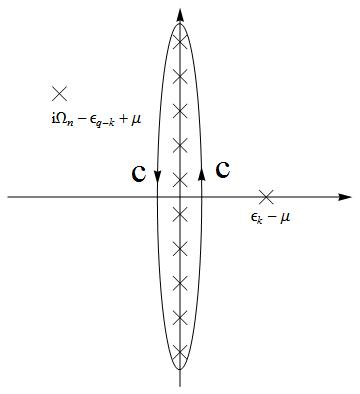
Failed to parse (SVG (MathML can be enabled via browser plugin): Invalid response ("Math extension cannot connect to Restbase.") from server "https://wikimedia.org/api/rest_v1/":): {\displaystyle \Rightarrow=\frac{1}{L^{D}}\frac{1}{\beta}\underset{\mathbf{k}}{\sum}\oint_{c}\frac{dz}{2\pi i}\frac{-1}{z-\varepsilon_{\mathbf{k}}+\mu}\times\frac{1}{z-i\Omega_{n}+\varepsilon_{\mathbf{q}-\mathbf{k}}-\mu}\frac{1}{e^{\beta z}+1}} .

Since Failed to parse (SVG (MathML can be enabled via browser plugin): Invalid response ("Math extension cannot connect to Restbase.") from server "https://wikimedia.org/api/rest_v1/":): {\displaystyle \frac{-1}{z-\varepsilon_{\mathbf{k}}+\mu}\times\frac{1}{z-i\Omega_{n}+\varepsilon_{\mathbf{q}-\mathbf{k}}-\mu}=\frac{1}{\varepsilon_{\mathbf{q}-\mathbf{k}}+\varepsilon_{\mathbf{k}}-2\mu-i\Omega_{n}}[\frac{1}{z-\varepsilon_{\mathbf{q}}+\mu}-\frac{1}{z-i\Omega_{n}+\varepsilon_{\mathbf{q}-\mathbf{k}}-\mu}]} ,

and change the integral path to

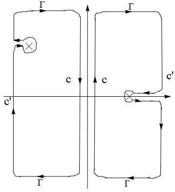
Failed to parse (SVG (MathML can be enabled via browser plugin): Invalid response ("Math extension cannot connect to Restbase.") from server "https://wikimedia.org/api/rest_v1/":): {\displaystyle \Rightarrow=-\frac{1}{L^{D}}\frac{1}{\beta}\underset{\mathbf{k}}{\sum}\frac{1}{\varepsilon_{\mathbf{q}-\mathbf{k}}+\varepsilon_{\mathbf{k}}-2\mu-i\Omega_{n}}[\frac{1}{e^{\beta(\varepsilon_{\mathbf{q}}-\mu)}+1}-\frac{1}{e^{\beta(-\varepsilon_{\mathbf{q}-\mathbf{k}}+\mu)}+1}]=\int\frac{d^{D}k}{(2\pi)^{D}}\frac{1}{\varepsilon_{\mathbf{q}}+\varepsilon_{\mathbf{q}-\mathbf{k}}-2\mu-i\Omega_{n}}[1-f(\varepsilon_{\mathbf{k}})-f(\varepsilon_{\mathbf{q}-\mathbf{k}})].}

In the static (Failed to parse (SVG (MathML can be enabled via browser plugin): Invalid response ("Math extension cannot connect to Restbase.") from server "https://wikimedia.org/api/rest_v1/":): {\displaystyle \ \Omega_{n}=0} ) and uniform (Failed to parse (SVG (MathML can be enabled via browser plugin): Invalid response ("Math extension cannot connect to Restbase.") from server "https://wikimedia.org/api/rest_v1/":): {\displaystyle \mathbf{q}=0} ) limit,Failed to parse (SVG (MathML can be enabled via browser plugin): Invalid response ("Math extension cannot connect to Restbase.") from server "https://wikimedia.org/api/rest_v1/":): {\displaystyle 1-2f(\varepsilon_{\mathbf{k}})=Tanh[\frac{\beta}{2}(\varepsilon_{\mathbf{k}}-\mu)]} .

Then Failed to parse (SVG (MathML can be enabled via browser plugin): Invalid response ("Math extension cannot connect to Restbase.") from server "https://wikimedia.org/api/rest_v1/":): {\displaystyle \chi_{p}(0,0)=\int\frac{d^{D}k}{(2\pi)^{D}}\frac{Tanh[\frac{\beta}{2}(\varepsilon_{\mathbf{k}}-\mu)]}{2(\varepsilon_{\mathbf{k}}-\mu)}} .

In low energy, integrate the energy in the shell near Fermi energy:

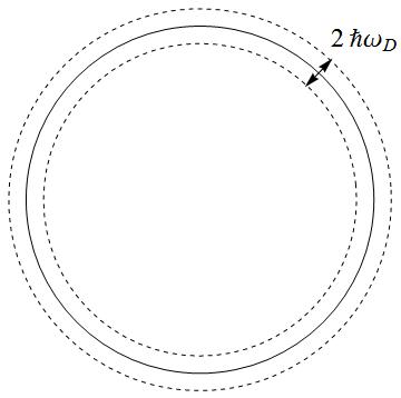
Failed to parse (SVG (MathML can be enabled via browser plugin): Invalid response ("Math extension cannot connect to Restbase.") from server "https://wikimedia.org/api/rest_v1/":): {\displaystyle \Rightarrow\chi_{p}(0,0)\cong N(0)\int_{\hbar\omega_{D}}^{-\hbar\omega_{D}}d\xi\frac{Tanh[\xi\beta/2]}{2\xi}\cong N(0)\int_{0}^{-\hbar\omega_{D}}d\xi\frac{Tanh[\xi\beta/2]}{\xi}=N(0)ln[\frac{2\hbar\omega_{D}e^{\gamma}}{\pi k_{B}T}].}

Then Failed to parse (SVG (MathML can be enabled via browser plugin): Invalid response ("Math extension cannot connect to Restbase.") from server "https://wikimedia.org/api/rest_v1/":): {\displaystyle \frac{1}{2}\left\langle S_{int.}^{2}\right\rangle _{0}=L^{D}\frac{1}{\beta}\chi_{p}(0,0)\underset{\Omega_{n},\mathbf{q}}{\sum}\Delta_{\mathbf{q}}^{*}(i\Omega_{n})\Delta_{\mathbf{q}}(i\Omega_{n})} .

If we ignore the higher order in the cumulant expansion,

Failed to parse (SVG (MathML can be enabled via browser plugin): Invalid response ("Math extension cannot connect to Restbase.") from server "https://wikimedia.org/api/rest_v1/":): {\displaystyle S_{eff}=-\underset{\mathbf{r}}{\sum}\int_{0}^{\beta}d\tau\frac{1}{g}\Delta_{\mathbf{q}}^{*}(i\Omega_{n})\Delta_{\mathbf{q}}(i\Omega_{n})-\frac{1}{2}\left\langle S_{int.}^{2}\right\rangle _{0}=\underset{\mathbf{r}}{\sum}\int_{0}^{\beta}d\tau[\frac{1}{\left|g\right|}-N(0)ln(\frac{2\hbar\omega_{D}e^{\gamma}}{\pi k_{B}T})]\Delta^{*}(\tau,\mathbf{r})\Delta(\tau,\mathbf{r})} .

Because the partition function Failed to parse (SVG (MathML can be enabled via browser plugin): Invalid response ("Math extension cannot connect to Restbase.") from server "https://wikimedia.org/api/rest_v1/":): {\displaystyle Z=\int D\Delta^{*}D\Delta e^{-S_{eff}(\Delta)}} , if we only consider the Failed to parse (SVG (MathML can be enabled via browser plugin): Invalid response ("Math extension cannot connect to Restbase.") from server "https://wikimedia.org/api/rest_v1/":): {\displaystyle \Delta} related factors.

The superconductivity phase transition temperature is the temperature makes Failed to parse (SVG (MathML can be enabled via browser plugin): Invalid response ("Math extension cannot connect to Restbase.") from server "https://wikimedia.org/api/rest_v1/":): {\displaystyle \frac{1}{\left|g\right|}-N(0)ln(\frac{2\hbar\omega_{D}e^{\gamma}}{\pi k_{B}T})=0} , which is Failed to parse (SVG (MathML can be enabled via browser plugin): Invalid response ("Math extension cannot connect to Restbase.") from server "https://wikimedia.org/api/rest_v1/":): {\displaystyle T_{c}=\frac{\hbar\omega_{D}}{k_{B}}\frac{2}{\pi}e^{\gamma}e^{-\frac{1}{N(0)\left|g\right|}}=1.134\frac{\hbar\omega_{D}}{k_{B}}e^{-\frac{1}{N(0)\left|g\right|}}} .

Beyond the critical temperature, the Failed to parse (SVG (MathML can be enabled via browser plugin): Invalid response ("Math extension cannot connect to Restbase.") from server "https://wikimedia.org/api/rest_v1/":): {\displaystyle \Delta} related factors in the partition function is just Failed to parse (SVG (MathML can be enabled via browser plugin): Invalid response ("Math extension cannot connect to Restbase.") from server "https://wikimedia.org/api/rest_v1/":): {\displaystyle 1} , the same as no cooper pair, which is normal state; below the critical temperature, the Failed to parse (SVG (MathML can be enabled via browser plugin): Invalid response ("Math extension cannot connect to Restbase.") from server "https://wikimedia.org/api/rest_v1/":): {\displaystyle \Delta} related factors in the partition function will diverge, which means superconductivity phase transition.

Finite Failed to parse (SVG (MathML can be enabled via browser plugin): Invalid response ("Math extension cannot connect to Restbase.") from server "https://wikimedia.org/api/rest_v1/":): {\displaystyle \vec{q}} (small) Failed to parse (SVG (MathML can be enabled via browser plugin): Invalid response ("Math extension cannot connect to Restbase.") from server "https://wikimedia.org/api/rest_v1/":): {\displaystyle \ (\Omega_n=0)}

Failed to parse (SVG (MathML can be enabled via browser plugin): Invalid response ("Math extension cannot connect to Restbase.") from server "https://wikimedia.org/api/rest_v1/":): {\displaystyle \chi_p (q,0)-\chi_p (0,0)=\frac{1}{L^D} \sum_k \frac{1}{\beta} \sum_{i\omega_n}\frac{-1}{i\omega_n-\epsilon_k+\mu}(\frac{1}{i\omega_n+\epsilon_{q-k}-\mu}-\frac{1}{i\omega_n+\epsilon_{-k}-\mu}) }

for small ${\vec {q}}$, $\epsilon _{q-k}=\epsilon _{-k}+q{\frac {\partial \epsilon _{\rho }}{\partial \rho }}|_{\rho =-k}=\epsilon _{\vec {k}}+{\vec {q}}\cdot {\vec {v}}_{-k}=\epsilon _{k}-{\vec {q}}\cdot {\vec {v}}_{k}$

and ${\frac {1}{i\omega _{n}+\epsilon _{k}-\mu -q\cdot v_{k}}}={\frac {1}{i\omega _{n}+\epsilon _{k}-\mu }}+{\frac {q\cdot v_{k}}{(i\omega _{n}+\epsilon _{k}-\mu )^{2}}}+{\frac {(q\cdot v_{k})^{2}}{(i\omega _{n}+\epsilon _{k}-\mu )^{3}}}$

Thus,

${\begin{aligned}\chi _{p}(q,0)-\chi _{p}(0,0)&={\frac {1}{L^{D}}}\sum _{k}{\frac {1}{\beta }}\sum _{i\omega _{n}}{\frac {-1}{i\omega _{n}-\epsilon _{k}+\mu }}\left({\frac {q\cdot v_{k}}{(i\omega _{n}+\epsilon _{k}-\mu )^{2}}}+{\frac {(q\cdot v_{k})^{2}}{(i\omega _{n}+\epsilon _{k}-\mu )^{3}}}+...\right)\\&={\frac {-1}{\beta }}\sum _{i}\omega _{n}\int {\frac {d^{D}k}{(2\pi )^{D}}}{\frac {({\vec {q}}\cdot {\vec {v}}_{k})^{2}}{(i\omega _{n}-\epsilon _{k}+\mu )(i\omega _{n}+\epsilon _{k}-\mu )^{3}}}\end{aligned}}$

Consider the states near the $\hbar \omega _{D}$ shell near fermi surface, we have

$\chi _{p}(q,0)-\chi _{p}(0,0)={\frac {1}{\beta }}\sum _{i\omega _{n}}\int {\frac {d\Omega _{F.S.}}{\Omega _{D}}}(q\cdot v_{F})^{2}\int _{-\infty }^{+\infty }d\xi N(\xi +\mu ){\frac {1}{(\xi -i\omega _{n})(\xi +i\omega _{n})^{3}}}$

where, $\ \xi =\epsilon _{k}-\mu$

and

${\begin{aligned}\int _{-\infty }^{+\infty }d\xi {\frac {1}{(\xi -i\omega _{n})(\xi +i\omega _{n})^{3}}}&={\frac {2\pi i}{(2i\omega _{n})^{3}}}\theta (\omega _{n})-{\frac {2\pi i}{(2i\omega _{n})^{3}}}\theta (-\omega _{n})\\&={\frac {2\pi i}{(2i|\omega |)^{3}}}\end{aligned}}$

So,

${\begin{aligned}\chi _{p}(q,0)-\chi _{p}(0,0)&={\frac {1}{\beta }}\sum _{i\omega _{n}}N(0)\int {\frac {d\Omega }{\Omega _{D}}}(q\cdot v_{F})^{2}{\frac {2\pi i}{(2i|\omega |)^{3}}}\\&=N(0)v_{F}^{2}|{\vec {q}}|^{2}\int {\frac {d\Omega }{\Omega _{D}}}(q\cdot v_{F})^{2}{\frac {1}{\beta }}\sum _{i\omega }{\frac {2\pi i}{-i8|{\frac {(2n+1)\pi }{\beta }}|^{3}}}\\&=-{\frac {1}{4}}N(0)v_{F}^{2}q^{2}(<({\hat {q}}\cdot {\hat {v_{F}}})>_{F.S.}){\frac {\beta ^{2}}{\pi ^{2}}}(\sum _{N=-\infty }^{+\infty }{\frac {1}{|2n+1|^{3}}})\end{aligned}}$

$\sum _{N=-\infty }^{+\infty }{\frac {1}{|2n+1|^{3}}}=\sum _{n=0}^{\infty }{\frac {2}{(2n+1)^{3}}}={\frac {2}{\pi }}{\frac {7\zeta (3)}{8}}$

where, $\ \zeta (3)$ is Riemann zeta function.

$<({\hat {q}}\cdot {\hat {v}}_{F})^{2}>_{F.S.}={\frac {1}{D}}$

For spherical F.S. in 3D,

Failed to parse (SVG (MathML can be enabled via browser plugin): Invalid response ("Math extension cannot connect to Restbase.") from server "https://wikimedia.org/api/rest_v1/":): {\displaystyle \int\frac{d\Omega}{\Omega_D}(\hat{q}\cdot\hat{v}_F)^2=\frac{2\pi}{4\pi}\int_{-1}^{1}dcos\theta cos^2\theta = \frac{1}{3} }

For circular F.S. in 2D,

Failed to parse (SVG (MathML can be enabled via browser plugin): Invalid response ("Math extension cannot connect to Restbase.") from server "https://wikimedia.org/api/rest_v1/":): {\displaystyle \int\frac{d\Omega}{\Omega_D}(\hat{q}\cdot\hat{v}_F)^2=\frac{1}{2\pi}\int_{0}^{2\pi}d\theta cos^2\theta = \frac{1}{2} }

Then

Failed to parse (SVG (MathML can be enabled via browser plugin): Invalid response ("Math extension cannot connect to Restbase.") from server "https://wikimedia.org/api/rest_v1/":): {\displaystyle \begin{align} \chi_p(q,0)-\chi_p(0,0) &=-\frac{1}{4}N(0)v_{F}^{2}q^{2}\frac{1}{D}\frac{\beta^{2}}{\pi^{2}}\frac{2}{\pi}\frac{7\zeta(3)}{8} \\ &=-N(0)\frac{7\zeta(3)}{16D\pi^{2}}q^{2}\frac{1}{\pi \hbar^{2}}\left(\frac{\hbar v_{F}}{k_{B}T}\right)^{2} \\ &\equiv-N(0)q^{2}\xi^{2} \end{align} }

So

Failed to parse (SVG (MathML can be enabled via browser plugin): Invalid response ("Math extension cannot connect to Restbase.") from server "https://wikimedia.org/api/rest_v1/":): {\displaystyle \begin{align} \frac{1}{2}\left\langle S_{int.}^{2}\right\rangle _{0}&=L^{D}\frac{1}{\beta}\underset{\Omega_{n},\mathbf{q}}{\sum}\chi_{p}(q,0)\Delta_{\mathbf{q}}^{*}(i\Omega_{n})\Delta_{\mathbf{q}}(i\Omega_{n}) \\ &=N(0)ln[\frac{2\hbar\omega_{D}e^{\gamma}}{\pi k_{B}T}]L^{D}\frac{1}{\beta}\underset{\Omega_{n},\mathbf{q}}{\sum}\Delta_{\mathbf{q}}^{*}(i\Omega_{n})\Delta_{\mathbf{q}}(i\Omega_{n})-L^{D}\frac{1}{\beta}\underset{\Omega_{n},\mathbf{q}}{\sum}N(0)q^{2}\xi^{2}\Delta_{\mathbf{q}}^{*}(i\Omega_{n})\Delta_{\mathbf{q}}(i\Omega_{n}) \end{align} } .

Failed to parse (SVG (MathML can be enabled via browser plugin): Invalid response ("Math extension cannot connect to Restbase.") from server "https://wikimedia.org/api/rest_v1/":): {\displaystyle S_{eff}=\underset{\mathbf{r}}{\sum}\int_{0}^{\beta}d\tau\left[\left(\frac{1}{\left|g\right|}-N(0)ln(\frac{2\hbar\omega_{D}e^{\gamma}}{\pi k_{B}T})\right)\Delta^{*}(\tau,\mathbf{r})\Delta(\tau,\mathbf{r})-N(0)\xi^{2}(\nabla\cdot\Delta^{*}(\tau,\mathbf{r}))(\nabla\cdot\Delta(\tau,\mathbf{r}))\right]} .

Note that the last term in the expression tells us that Failed to parse (SVG (MathML can be enabled via browser plugin): Invalid response ("Math extension cannot connect to Restbase.") from server "https://wikimedia.org/api/rest_v1/":): {\displaystyle S_{eff} } would increase if gradient of $\Delta$ is not zero.

Note that the above expression has a one-one correspondant to the Giznburg-Landau functional:

$F=\int d^{D}r\left[\alpha (T-T_{c})|\Psi ({\vec {r}})|^{2}+{\frac {\hbar ^{2}}{2m^{*}}}|\nabla \Psi ({\vec {r}})|^{2}\right]$,

here $\ \Psi ({\vec {r}})$ corresponds to $\ {\frac {\Delta (\tau ,{\vec {r}})}{|g|N(0)a_{0}}}$ in $S_{eff}$.

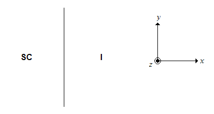
Little Parks experiment

Refer to the fig, a thin shell of superconductor with radius R is shown and a small uniform magnetic field is passing through the hollow center of the cylinder. The experiment intends to show the variation of the critical temperature with change of the magnetic field passing through the hollow superconductor cylinder.

Before showing it, we first have to rewrite the Giznburg-Landau functional to make it taken the presence of magnetic field into account. Hamiltonian for a free electron moving in a magnetic field can be written as:

${\frac {1}{2m}}(p+{\frac {eA}{c}})^{2}\psi +V\psi =E\psi$

The physical observable magnetic field B would remain the same if we choose a different vector potential $A\rightarrow A+\nabla \chi$ (ie perform gauge transformation). To maintain the same eigen-energy E which is observable, the wave function have to undergo a phase change: $\psi \rightarrow e^{i\phi }\psi$ where $\phi ={\frac {e}{c\hbar }}\chi$

Now in our Hamiltonian, the wave function is arranged as $\Delta ^{*}(\tau ,{\vec {r}})\psi _{\uparrow }(\tau ,{\vec {r}})\psi _{\downarrow }(\tau ,{\vec {r}})+\Delta (\tau ,{\vec {r}})\psi _{\downarrow }^{\dagger }(\tau ,{\vec {r}})\psi _{\uparrow }^{\dagger }(\tau ,{\vec {r}})$

since $\psi \rightarrow e^{i\phi }\psi$, so if we want the Hamiltonian to remind the same, $\ \Delta$ has to transform as Failed to parse (SVG (MathML can be enabled via browser plugin): Invalid response ("Math extension cannot connect to Restbase.") from server "https://wikimedia.org/api/rest_v1/":): {\displaystyle \Delta \rightarrow e^{-2i\phi}\Delta }

Since Failed to parse (SVG (MathML can be enabled via browser plugin): Invalid response ("Math extension cannot connect to Restbase.") from server "https://wikimedia.org/api/rest_v1/":): {\displaystyle \ \Delta } corresponds to Failed to parse (SVG (MathML can be enabled via browser plugin): Invalid response ("Math extension cannot connect to Restbase.") from server "https://wikimedia.org/api/rest_v1/":): {\displaystyle \ \Psi } in the Giznburg-Landau functional, so the Giznburg-Landau functional is modified as

Failed to parse (SVG (MathML can be enabled via browser plugin): Invalid response ("Math extension cannot connect to Restbase.") from server "https://wikimedia.org/api/rest_v1/":): {\displaystyle F=\int d^{D}r\left[ \alpha (T-T_{c}) |\Psi(\vec{r})|^{2}+\frac{1}{2m^{*}}| ( \frac{\hbar \nabla}{i} - \frac{2e}{c}A(\vec{r}) ) \Psi(\vec{r})|^{2} \right] }

choose symmetric gauge: Failed to parse (SVG (MathML can be enabled via browser plugin): Invalid response ("Math extension cannot connect to Restbase.") from server "https://wikimedia.org/api/rest_v1/":): {\displaystyle \vec{A}=\frac{1}{2}\vec{H}\times\vec{r}=\frac{1}{2}Hr\hat{\phi} }

In cylindrical coordinate: Failed to parse (SVG (MathML can be enabled via browser plugin): Invalid response ("Math extension cannot connect to Restbase.") from server "https://wikimedia.org/api/rest_v1/":): {\displaystyle \vec{\nabla}=\hat{r}\frac{\partial}{\partial r} + \frac{\hat{\phi}}{r}\frac{\partial}{\partial \phi} + \hat{z}\frac{\partial}{\partial z} }

define unit flux as Failed to parse (SVG (MathML can be enabled via browser plugin): Invalid response ("Math extension cannot connect to Restbase.") from server "https://wikimedia.org/api/rest_v1/":): {\displaystyle \Phi_{0}=\frac{hc}{2e} }

define fluxoid as Failed to parse (SVG (MathML can be enabled via browser plugin): Invalid response ("Math extension cannot connect to Restbase.") from server "https://wikimedia.org/api/rest_v1/":): {\displaystyle \Phi(R) = \pi HR^{2}\ } , so we have

Failed to parse (SVG (MathML can be enabled via browser plugin): Invalid response ("Math extension cannot connect to Restbase.") from server "https://wikimedia.org/api/rest_v1/":): {\displaystyle \begin{align} F&=\int d^{D}r\left[ \alpha (T-T_{c})|\Psi(\vec{r})|^{2} +\frac{\hbar^{2}}{2m^{*}}| (\frac{1}{R}\frac{\partial}{\partial \phi} - \frac{ie}{\hbar c} HR )\Psi(\vec{r}) |^{2}+ \frac{\hbar^{2}}{2m^{*}}|\frac{\partial}{\partial z} \Psi(\vec{r}) |^{2} \right] \\ &=\int d^{D}r\left[ \alpha (T-T_{c})|\Psi(\vec{r})|^{2} +\frac{\hbar^{2}}{2m^{*}R^{2}}| (\frac{\partial}{\partial \phi} - \frac{i\Phi}{\Phi_{0}} )\Psi(\vec{r}) |^{2} \right] \\ \end{align} }

When Failed to parse (SVG (MathML can be enabled via browser plugin): Invalid response ("Math extension cannot connect to Restbase.") from server "https://wikimedia.org/api/rest_v1/":): {\displaystyle \Phi = N\Phi_{0}\ } , the critical temperature will remain the same and the phase of Failed to parse (SVG (MathML can be enabled via browser plugin): Invalid response ("Math extension cannot connect to Restbase.") from server "https://wikimedia.org/api/rest_v1/":): {\displaystyle \Psi\ } is changed as Failed to parse (SVG (MathML can be enabled via browser plugin): Invalid response ("Math extension cannot connect to Restbase.") from server "https://wikimedia.org/api/rest_v1/":): {\displaystyle \Psi \rightarrow e^{iN\phi} \Psi } . When Failed to parse (SVG (MathML can be enabled via browser plugin): Invalid response ("Math extension cannot connect to Restbase.") from server "https://wikimedia.org/api/rest_v1/":): {\displaystyle \Phi \neq N\Phi_{0}\ } , the critical temperature is found to vary as Failed to parse (SVG (MathML can be enabled via browser plugin): Invalid response ("Math extension cannot connect to Restbase.") from server "https://wikimedia.org/api/rest_v1/":): {\displaystyle T_{c}^{new}=T_{c}- \frac{\hbar^{2}}{2m^{*}R^{2}\alpha}\left (N-\frac{\Phi}{\Phi_{0}}\right )^{2}} . See the fig.

Microscopic derivation of the Giznburg-Landau functional

Let us consider the model of a metal close to the transition to the superconducting state. A complete description of its thermodynamic properties can be done through the calculation of the partition function.

The classical part of the Hamiltonian in the partition function, dependent of bosonic fields, may be chosen in the spirit of the Landauer theory of phase transition. However, in view of the space dependence of wave functions, Ginzberg and Landauer included in it additionally the first non vanishing term of the expansion over the gradient of the fluctuation field. Symmetry analysis shows that it should be quadratic. The weakness of the field coordinate dependence permits to omit the high-order terms of such an expansion. Therefore, the classical part of the Hamiltonian of a metal close to a superconducting transition related to the presence of the fluctuation Cooper pairs in it (the so called Ginzberg-Landauer functional)can be written as

Failed to parse (SVG (MathML can be enabled via browser plugin): Invalid response ("Math extension cannot connect to Restbase.") from server "https://wikimedia.org/api/rest_v1/":): {\displaystyle F[\psi(r)]=F_{n}+\int dV\{a\mid\psi(r)\mid^{2}+\frac{b}{2}\mid\psi(r)\mid^{4}+\frac{1}{4m}\mid\nabla\psi(r)\mid^{2}\}}

We already got the quadratic terms in the Ginzberg-Landauer by expanding Failed to parse (SVG (MathML can be enabled via browser plugin): Invalid response ("Math extension cannot connect to Restbase.") from server "https://wikimedia.org/api/rest_v1/":): {\displaystyle <e^{-S_{int}}>} to the second order, and we are going to go the higher order. As we discussed, we expect that this term will be a negative value to keep Failed to parse (SVG (MathML can be enabled via browser plugin): Invalid response ("Math extension cannot connect to Restbase.") from server "https://wikimedia.org/api/rest_v1/":): {\displaystyle S_{eff}} as a negative value under Failed to parse (SVG (MathML can be enabled via browser plugin): Invalid response ("Math extension cannot connect to Restbase.") from server "https://wikimedia.org/api/rest_v1/":): {\displaystyle T_{c}} . To catch this goal we start with the partition function:

Failed to parse (SVG (MathML can be enabled via browser plugin): Invalid response ("Math extension cannot connect to Restbase.") from server "https://wikimedia.org/api/rest_v1/":): {\displaystyle Z=Z_{0}< e^{-S_{int}} >}

where Failed to parse (SVG (MathML can be enabled via browser plugin): Invalid response ("Math extension cannot connect to Restbase.") from server "https://wikimedia.org/api/rest_v1/":): {\displaystyle Z_{0}=\int D\psi ^{*} D\psi D\Delta ^{*} D\Delta e^{-(S_{\Delta} +S_{0})}}

we can expand this average for smallFailed to parse (SVG (MathML can be enabled via browser plugin): Invalid response ("Math extension cannot connect to Restbase.") from server "https://wikimedia.org/api/rest_v1/":): {\displaystyle \Delta} nearFailed to parse (SVG (MathML can be enabled via browser plugin): Invalid response ("Math extension cannot connect to Restbase.") from server "https://wikimedia.org/api/rest_v1/":): {\displaystyle T_{c}} , for this perpose we can assume asecond order phase transition so that it increases continiously from zero to finite number after Failed to parse (SVG (MathML can be enabled via browser plugin): Invalid response ("Math extension cannot connect to Restbase.") from server "https://wikimedia.org/api/rest_v1/":): {\displaystyle T_{c}}

we need to calculate the average of Failed to parse (SVG (MathML can be enabled via browser plugin): Invalid response ("Math extension cannot connect to Restbase.") from server "https://wikimedia.org/api/rest_v1/":): {\displaystyle e^{-s_{int}}} which can be calculated by Tylor expansion:

Failed to parse (SVG (MathML can be enabled via browser plugin): Invalid response ("Math extension cannot connect to Restbase.") from server "https://wikimedia.org/api/rest_v1/":): {\displaystyle e^{-S_{int}}=<-S_{int}+\frac{1}{2}S_{int}^{2}-\frac{1}{3}S_{int}^{3}+\frac{1}{4!}S_{int}^{4}+...>}

=Failed to parse (SVG (MathML can be enabled via browser plugin): Invalid response ("Math extension cannot connect to Restbase.") from server "https://wikimedia.org/api/rest_v1/":): {\displaystyle 1-<S_{int}>+\frac{1}{2} < S_{int}^{2}> -\frac{1}{3!}< S_{int}^{2}> +\frac{1}{4!}< S_{int}^{4}> +...}

the odd power terms are zero because Failed to parse (SVG (MathML can be enabled via browser plugin): Invalid response ("Math extension cannot connect to Restbase.") from server "https://wikimedia.org/api/rest_v1/":): {\displaystyle <\psi _{\uparrow}(r,\tau )\psi _{\downarrow}(r,\tau ) > =0 }

Failed to parse (SVG (MathML can be enabled via browser plugin): Invalid response ("Math extension cannot connect to Restbase.") from server "https://wikimedia.org/api/rest_v1/":): {\displaystyle =e^{\frac{1}{2}< S_{int}^{2}>}e^{\frac{1}{4!}< S_{int}^{4}>-\lambda }}

if we expand these two terms in to the second order the following expression can be got:

Failed to parse (SVG (MathML can be enabled via browser plugin): Invalid response ("Math extension cannot connect to Restbase.") from server "https://wikimedia.org/api/rest_v1/":): {\displaystyle (1+\frac{1}{2} < S_{int}^{2}>+\frac{1}{2}(<\frac{1}{2} S_{int}^{2}>)^{2} +...)(1+\frac{1}{4!}< S_{int}^{4}>+...)}

Failed to parse (SVG (MathML can be enabled via browser plugin): Invalid response ("Math extension cannot connect to Restbase.") from server "https://wikimedia.org/api/rest_v1/":): {\displaystyle =1+\frac{1}{2} < S_{int}^{2}>+\frac{1}{8}(< S_{int}^{2}>)^{2} +...)+\frac{1}{4!}< S_{int}^{4}>-\lambda +...}

Failed to parse (SVG (MathML can be enabled via browser plugin): Invalid response ("Math extension cannot connect to Restbase.") from server "https://wikimedia.org/api/rest_v1/":): {\displaystyle \lambda} can be choosed in such a way .......

so, Failed to parse (SVG (MathML can be enabled via browser plugin): Invalid response ("Math extension cannot connect to Restbase.") from server "https://wikimedia.org/api/rest_v1/":): {\displaystyle \lambda =\frac{1}{8}< S_{int}^{2}> ^{2} }

$=e^{{\frac {1}{2}}<S_{int}^{2}>+{\frac {1}{4!}}(<S_{int}^{4}>-3<S_{int}^{2}>^{2})+...}$

according to the expression we got before:

$S_{int}={\frac {L^{D}}{\beta ^{2}}}\sum _{\omega _{n},\Omega _{n}}\sum _{k,q}[\Delta _{q}^{*}(i\Omega _{n})\psi _{\downarrow }(i\Omega _{n}-i\omega _{n}),{\vec {q}}-{\vec {k}})\psi _{\uparrow }(i\omega _{n},k)+\Delta _{q}(i\Omega _{n})\psi _{\uparrow }^{\dagger }(i\omega _{n},k)\psi _{\downarrow }^{\dagger }(i\Omega _{n}-i\omega _{n}),{\vec {q}}-{\vec {k}})]$

let's write $S_{int}$ in terems od $a$ for simplification. where

$a=\int \Delta ^{*}(1)\psi _{\downarrow }(1)\psi _{\uparrow }(1)+\Delta (1)\psi _{\downarrow }^{*}(1)\psi _{\uparrow }^{*}(1)$

$a_{1}$ is a couple grassman number, so we do not need to be worry about the sign when these terms comute with other terms.

$<S_{int}^{4}>=\int _{1234}<(a_{1}^{*}+a_{1})(a_{2}^{*}+a_{2})(a_{3}^{*}+a_{3})(a_{4}^{*}+a_{4})>$

$=(<a_{1}^{*}a_{2}^{*}a_{3}a_{4}>+<a_{1}^{*}a_{2}a_{3}^{*}a_{4}>+<a_{1}^{*}a_{2}a_{3}a_{4}^{*}>+<a_{1}a_{2}^{*}a_{3}^{*}a_{4}>+<a_{1}a_{2}^{*}a_{3}a_{4}^{*}>)$

$=6<a_{1}^{*}a_{2}^{*}a_{3}a_{4}>=6\int _{1234}\Delta ^{*}(1)\Delta ^{*}(2)\Delta (3)\Delta (4)<\psi _{\downarrow }(1)\psi _{\uparrow }(1)\psi _{\downarrow }(2)\psi _{\uparrow }(2)\psi _{\downarrow }^{*}(3)\psi _{\uparrow }^{*}(3)\psi _{\downarrow }^{*}(4)\psi _{\uparrow }^{*}(4)>$

$3<S_{int}^{2}>^{2}=3\int _{1,2}2<a_{1}^{*}a_{2}>\int _{3,4}2<a_{3}^{*}a_{4}>=12\int _{1,2,3,4}\Delta ^{*}(1)\Delta ^{*}(2)\Delta (3)\Delta (4)<\psi _{\downarrow }(1)\psi _{\uparrow }(1)\psi _{\uparrow }^{*}(3)\psi _{\downarrow }^{*}(3)><\psi _{\downarrow }(2)\psi _{\uparrow }(2)\psi _{\uparrow }^{*}(4)\psi _{\downarrow }^{*}(4)>$

$-2G(2-3)G(2-4)G(1-4)G(1-3)=-12\int _{1,2,3,4}\Delta ^{*}(1)\Delta _{*}(2)\Delta (3)\Delta (4)G(2-3)G(2-4)G(1-4)G(1-3)$

Recall the Fourier transform of one body Green function is:

$G(2-3)=<\psi (r_{2},\tau _{2})\psi ^{*}(r_{3},\tau _{3})>={\frac {1}{\beta }}\sum _{\omega _{n}}{\frac {1}{L^{D}}}\sum _{k}e^{-i\omega _{n}(\tau _{2}-\tau _{3})}e^{ik.(r_{2}-r_{3})}{\frac {1}{-i\omega _{n}+\epsilon _{k}-\mu }}$

To seek solution of which are Failed to parse (SVG (MathML can be enabled via browser plugin): Invalid response ("Math extension cannot connect to Restbase.") from server "https://wikimedia.org/api/rest_v1/":): {\displaystyle \tau} independent using Feynman diagram

Failed to parse (SVG (MathML can be enabled via browser plugin): Invalid response ("Math extension cannot connect to Restbase.") from server "https://wikimedia.org/api/rest_v1/":): {\displaystyle \frac{1}{\beta ^{4}}\sum_{\omega _{{n}_{1}}}...\sum_{\omega _{{n}_{4}}}\int_{0}^\beta {d\tau_{1}}\int_{0}^\beta {d\tau_{2}} \int_{0}^\beta {d\tau_{3}} \int_{0}^\beta {d\tau_{4}}e^{-i\omega _{{n}_{1}}(\tau _{1}-\tau _{3})} e^{-i\omega _{{n}_{2}}(\tau _{1}-\tau _{4})}e^{-i\omega _{{n}_{3}}(\tau _{2}-\tau _{3})}e^{-i\omega _{{n}_{4}}(\tau _{2}-\tau _{4})} G(i\omega _{{n}_{1}},r_{1}-r_{3})\times}

Failed to parse (SVG (MathML can be enabled via browser plugin): Invalid response ("Math extension cannot connect to Restbase.") from server "https://wikimedia.org/api/rest_v1/":): {\displaystyle G(i\omega _{{n}_{2}},r_{1}-r_{4})G(i\omega _{{n}_{3}},r_{2}-r_{3})G(i\omega _{{n}_{4}},r_{2}-r_{4})}

after getting integration over Failed to parse (SVG (MathML can be enabled via browser plugin): Invalid response ("Math extension cannot connect to Restbase.") from server "https://wikimedia.org/api/rest_v1/":): {\displaystyle \tau_{1}} we will get Failed to parse (SVG (MathML can be enabled via browser plugin): Invalid response ("Math extension cannot connect to Restbase.") from server "https://wikimedia.org/api/rest_v1/":): {\displaystyle \beta \delta (\omega _{n_{1}},-\omega _{n_{2}}) } and similarly by getting integration over Failed to parse (SVG (MathML can be enabled via browser plugin): Invalid response ("Math extension cannot connect to Restbase.") from server "https://wikimedia.org/api/rest_v1/":): {\displaystyle \tau_{2}} we have Failed to parse (SVG (MathML can be enabled via browser plugin): Invalid response ("Math extension cannot connect to Restbase.") from server "https://wikimedia.org/api/rest_v1/":): {\displaystyle \beta \delta (\omega _{n_{3}},-\omega _{n_{4}}) }

So, the final result can be written: Failed to parse (SVG (MathML can be enabled via browser plugin): Invalid response ("Math extension cannot connect to Restbase.") from server "https://wikimedia.org/api/rest_v1/":): {\displaystyle \sum_{i\omega _{n}}G(i\omega _{n},r_{1}-r_{3}G(-i\omega _{n},r_{2}-r_{3})G(-i\omega _{n},r_{1}-r_{4})G(i\omega _{n},r_{2}-r_{4}) }

Now, we wish to perform gradiant expansion:

Failed to parse (SVG (MathML can be enabled via browser plugin): Invalid response ("Math extension cannot connect to Restbase.") from server "https://wikimedia.org/api/rest_v1/":): {\displaystyle \Delta ^{\ast }(1)=\Delta ^{\ast }(\frac{r_{1}+r_{4}}{2}+\frac{r_{1}-r_{4}}{2})=\Delta ^{\ast }(\frac{r_{1}+r_{4}}{2})+(\frac{r_{1}-r_{4}}{2})\nabla\Delta^{\ast }(\frac{r_{1}+r_{4}}{2})+... }

Failed to parse (SVG (MathML can be enabled via browser plugin): Invalid response ("Math extension cannot connect to Restbase.") from server "https://wikimedia.org/api/rest_v1/":): {\displaystyle \Delta ^{\ast }(2)=\Delta ^{\ast }(\frac{r_{2}+r_{3}}{2}+\frac{r_{2}-r_{3}}{2})=\Delta ^{\ast }(\frac{r_{2}+r_{3}}{2})+(\frac{r_{2}-r_{3}}{2})\nabla\Delta^{\ast }(\frac{r_{2}+r_{3}}{2})+... } Failed to parse (SVG (MathML can be enabled via browser plugin): Invalid response ("Math extension cannot connect to Restbase.") from server "https://wikimedia.org/api/rest_v1/":): {\displaystyle -12\int d^{D}R_{1,4}d^{D}R_{2,3}d^{D}\mu _{1,4}d^{D}\mu_{2,3}\Delta ^{\ast }(R_{1,4})\Delta ^{\ast }(R_{2,3})\Delta (R_{2,3}) \Delta (R_{1,4})\sum_{\omega_{n}}G(i\omega_{n},R_{1,4}-R_{2,3}+\frac{1}{2}(\mu _{1,4}+\mu _{2,3}))}

where:

Failed to parse (SVG (MathML can be enabled via browser plugin): Invalid response ("Math extension cannot connect to Restbase.") from server "https://wikimedia.org/api/rest_v1/":): {\displaystyle R=\frac{1}{2}(R_{1,4}+R_{2,3})}

Failed to parse (SVG (MathML can be enabled via browser plugin): Invalid response ("Math extension cannot connect to Restbase.") from server "https://wikimedia.org/api/rest_v1/":): {\displaystyle \mu =R_{1,4}-R_{2,3} }

Failed to parse (SVG (MathML can be enabled via browser plugin): Invalid response ("Math extension cannot connect to Restbase.") from server "https://wikimedia.org/api/rest_v1/":): {\displaystyle r_{1}-r_{3}=\frac{1}{2}(\mu _{1,4}+\mu_{2,3})+\mu}

Failed to parse (SVG (MathML can be enabled via browser plugin): Invalid response ("Math extension cannot connect to Restbase.") from server "https://wikimedia.org/api/rest_v1/":): {\displaystyle r_{2}-r_{4}=\frac{1}{2}(\mu _{1,4}+\mu_{2,3})-\mu}

Failed to parse (SVG (MathML can be enabled via browser plugin): Invalid response ("Math extension cannot connect to Restbase.") from server "https://wikimedia.org/api/rest_v1/":): {\displaystyle \simeq -12\int d^{D}R d^{D}\mu d^{D}\mu_{1.4}d^{D}\mu_{2,3}\Delta ^{\ast }(R)\Delta^{\ast } (R)\Delta (R)\Delta (R)\sum_{\omega _n}G(i\omega _{n},\mu +\frac{1}{2}(\mu_{1,4}+\mu _{2,3}))G(-i\omega _{n},\mu _{1,4})G(-i\omega _{n},\mu _{2,3})G(i\omega _{n},\mu +\frac{1}{2}(\mu_{1,4}+\mu _{2,3}))}

integrate overFailed to parse (SVG (MathML can be enabled via browser plugin): Invalid response ("Math extension cannot connect to Restbase.") from server "https://wikimedia.org/api/rest_v1/":): {\displaystyle \mu} gives us Failed to parse (SVG (MathML can be enabled via browser plugin): Invalid response ("Math extension cannot connect to Restbase.") from server "https://wikimedia.org/api/rest_v1/":): {\displaystyle l^{D}} Failed to parse (SVG (MathML can be enabled via browser plugin): Invalid response ("Math extension cannot connect to Restbase.") from server "https://wikimedia.org/api/rest_v1/":): {\displaystyle \delta_{k_{1},k_{4}}}

and similarly Failed to parse (SVG (MathML can be enabled via browser plugin): Invalid response ("Math extension cannot connect to Restbase.") from server "https://wikimedia.org/api/rest_v1/":): {\displaystyle \mu_{1,4}} Failed to parse (SVG (MathML can be enabled via browser plugin): Invalid response ("Math extension cannot connect to Restbase.") from server "https://wikimedia.org/api/rest_v1/":): {\displaystyle l^{D}} Failed to parse (SVG (MathML can be enabled via browser plugin): Invalid response ("Math extension cannot connect to Restbase.") from server "https://wikimedia.org/api/rest_v1/":): {\displaystyle \delta_{k_{1},-k_{2}}}

Failed to parse (SVG (MathML can be enabled via browser plugin): Invalid response ("Math extension cannot connect to Restbase.") from server "https://wikimedia.org/api/rest_v1/":): {\displaystyle \mu_{2,3}} Failed to parse (SVG (MathML can be enabled via browser plugin): Invalid response ("Math extension cannot connect to Restbase.") from server "https://wikimedia.org/api/rest_v1/":): {\displaystyle l^{D}} Failed to parse (SVG (MathML can be enabled via browser plugin): Invalid response ("Math extension cannot connect to Restbase.") from server "https://wikimedia.org/api/rest_v1/":): {\displaystyle \delta_{k_{1},-k_{3}}}

Starting from the microscopic model, we found that Failed to parse (SVG (MathML can be enabled via browser plugin): Invalid response ("Math extension cannot connect to Restbase.") from server "https://wikimedia.org/api/rest_v1/":): {\displaystyle Z\backsimeq Z_{0}\int D\Delta*D\Delta e^{-S_{eff}} } , where the Failed to parse (SVG (MathML can be enabled via browser plugin): Invalid response ("Math extension cannot connect to Restbase.") from server "https://wikimedia.org/api/rest_v1/":): {\displaystyle 4^{th}} order in Failed to parse (SVG (MathML can be enabled via browser plugin): Invalid response ("Math extension cannot connect to Restbase.") from server "https://wikimedia.org/api/rest_v1/":): {\displaystyle \Delta} , and keeping only quadratic qradient terms, we have:

Failed to parse (SVG (MathML can be enabled via browser plugin): Invalid response ("Math extension cannot connect to Restbase.") from server "https://wikimedia.org/api/rest_v1/":): {\displaystyle S_{eff}=\frac{1}{k_{B}T}\sum_{r}\left[\underset{A}{\underbrace{\left(\frac{1}{|g|}-N(0)In\left[\frac{2\hbar\omega_{D}e^{\gamma_{E}}}{\pi k_{B}T}\right]\right)}}|\Delta(r)|^{2}+N(0)\xi^{2}(\nabla\Delta*(r)).(\nabla\Delta(r))+\frac{1}{2}\underset{B}{\underbrace{\frac{7\zeta(3)N(0)}{8\pi^{2}k_{B}^{2}T^{2}}}}|\Delta(r)|^{4}\right]}

We can use this expression to make quantitative experimental predictions. The path integral over Failed to parse (SVG (MathML can be enabled via browser plugin): Invalid response ("Math extension cannot connect to Restbase.") from server "https://wikimedia.org/api/rest_v1/":): {\displaystyle \Delta} is still imposible to carry out exactly, despite our approximations for Failed to parse (SVG (MathML can be enabled via browser plugin): Invalid response ("Math extension cannot connect to Restbase.") from server "https://wikimedia.org/api/rest_v1/":): {\displaystyle S_{eff}} , because Failed to parse (SVG (MathML can be enabled via browser plugin): Invalid response ("Math extension cannot connect to Restbase.") from server "https://wikimedia.org/api/rest_v1/":): {\displaystyle S_{eff}} contains quartic terms in Failed to parse (SVG (MathML can be enabled via browser plugin): Invalid response ("Math extension cannot connect to Restbase.") from server "https://wikimedia.org/api/rest_v1/":): {\displaystyle \Delta} and so we are not dealing with a Gaussian integral. The approximation strategy whic we will pursue is called saddle point approxiation, which in our contetxt means that we will expand teh integrand about a solution which minimizes S_{eff} with respect to Failed to parse (SVG (MathML can be enabled via browser plugin): Invalid response ("Math extension cannot connect to Restbase.") from server "https://wikimedia.org/api/rest_v1/":): {\displaystyle \Delta} . What we end up doing is replacing Z with Failed to parse (SVG (MathML can be enabled via browser plugin): Invalid response ("Math extension cannot connect to Restbase.") from server "https://wikimedia.org/api/rest_v1/":): {\displaystyle Z\sim Z_{0}e^{-S_{eff}[\Delta_{min}]}} , where Failed to parse (SVG (MathML can be enabled via browser plugin): Invalid response ("Math extension cannot connect to Restbase.") from server "https://wikimedia.org/api/rest_v1/":): {\displaystyle \Delta_{min}} is determined fromFailed to parse (SVG (MathML can be enabled via browser plugin): Invalid response ("Math extension cannot connect to Restbase.") from server "https://wikimedia.org/api/rest_v1/":): {\displaystyle \left|\frac{\delta S_{eff}}{\delta\Delta^{*}}\right|_{\Delta=\Delta_{min}}=0} At this point, let's seek uniform solutions to their equations, in whcih case we can drop the gradient terms in Failed to parse (SVG (MathML can be enabled via browser plugin): Invalid response ("Math extension cannot connect to Restbase.") from server "https://wikimedia.org/api/rest_v1/":): {\displaystyle S_{eff}}  : Failed to parse (SVG (MathML can be enabled via browser plugin): Invalid response ("Math extension cannot connect to Restbase.") from server "https://wikimedia.org/api/rest_v1/":): {\displaystyle \frac{\delta S_{eff}}{\delta\Delta^{*}}=\frac{L^{D}}{k_{B}T}\left(A\Delta+B\Delta\Delta^{*}\Delta\right)} where: Failed to parse (SVG (MathML can be enabled via browser plugin): Invalid response ("Math extension cannot connect to Restbase.") from server "https://wikimedia.org/api/rest_v1/":): {\displaystyle A=\frac{1}{|g|}-N(0)ln\left(\frac{\hbar\omega_{D}}{k_{B}T}\frac{2e\gamma}{\pi}\right)} and Failed to parse (SVG (MathML can be enabled via browser plugin): Invalid response ("Math extension cannot connect to Restbase.") from server "https://wikimedia.org/api/rest_v1/":): {\displaystyle B=\frac{7\zeta(3)}{8\pi}\frac{N(0)}{k_{B}^{2}T^{2}}}

Note that for : Failed to parse (SVG (MathML can be enabled via browser plugin): Invalid response ("Math extension cannot connect to Restbase.") from server "https://wikimedia.org/api/rest_v1/":): {\displaystyle T>T_{C}\qquad A>0,B>0} and Failed to parse (SVG (MathML can be enabled via browser plugin): Invalid response ("Math extension cannot connect to Restbase.") from server "https://wikimedia.org/api/rest_v1/":): {\displaystyle T<T_{C}\qquad A<0,B>0}

So Failed to parse (SVG (MathML can be enabled via browser plugin): Invalid response ("Math extension cannot connect to Restbase.") from server "https://wikimedia.org/api/rest_v1/":): {\displaystyle A\Delta_{min}+B\Delta_{min}^{3}=0} ,

Failed to parse (SVG (MathML can be enabled via browser plugin): Invalid response ("Math extension cannot connect to Restbase.") from server "https://wikimedia.org/api/rest_v1/":): {\displaystyle \Delta_{min}=0, \;T>T_{C}} and

Failed to parse (SVG (MathML can be enabled via browser plugin): Invalid response ("Math extension cannot connect to Restbase.") from server "https://wikimedia.org/api/rest_v1/":): {\displaystyle \Delta_{min}=\sqrt{\frac{-A}{B}},\; T<T_{C} } .

Failed to parse (SVG (MathML can be enabled via browser plugin): Invalid response ("Math extension cannot connect to Restbase.") from server "https://wikimedia.org/api/rest_v1/":): {\displaystyle S_{eff}[\Delta_{min}]=\frac{L^{D}}{k_{B}T}\left(A\Delta_{min}^{2}+\frac{1}{2}B\Delta_{min}^{4}\right)}

Failed to parse (SVG (MathML can be enabled via browser plugin): Invalid response ("Math extension cannot connect to Restbase.") from server "https://wikimedia.org/api/rest_v1/":): {\displaystyle T>T_{C};\quad S_{eff}[\Delta_{min}]=0} ,

Failed to parse (SVG (MathML can be enabled via browser plugin): Invalid response ("Math extension cannot connect to Restbase.") from server "https://wikimedia.org/api/rest_v1/":): {\displaystyle T<T_{C};\quad S_{eff}[\Delta_{min}]=\left(A\frac{-A}{B}+\frac{1}{2}B\frac{A^{2}}{B^{2}}\right)\frac{L^{D}}{k_{B}T}=\frac{-A^{2}}{2B}\frac{L^{D}}{k_{B}T}}

Since, we now have the approximate expression for the partition function we can calculate thermodynamic physical properties. the one we will focus on is the specific heat. Recall that, Failed to parse (SVG (MathML can be enabled via browser plugin): Invalid response ("Math extension cannot connect to Restbase.") from server "https://wikimedia.org/api/rest_v1/":): {\displaystyle Z=e^{-\beta F}=\sum_{n}e^{-\beta E_{n}}\Longrightarrow<E>=\frac{1}{Z}\sum_{n}E_{n}e^{-\beta E_{n}}=-\frac{\partial}{\partial\beta}lnZ =-\frac{\partial}{\partial\beta}lne^{-\beta F}=\frac{\partial}{\partial\beta}\left(\beta F\right)=F+\beta\frac{\partial F}{\partial\beta}}

Failed to parse (SVG (MathML can be enabled via browser plugin): Invalid response ("Math extension cannot connect to Restbase.") from server "https://wikimedia.org/api/rest_v1/":): {\displaystyle =\frac{\partial F}{\partial T}+\frac{\partial\beta}{\partial T}\frac{\partial F}{\partial\beta}+\beta\frac{\partial}{\partial T}\frac{\partial F}{\partial\beta}}

$=2{\frac {\partial F}{\partial T}}+\beta {\frac {\partial }{\partial T}}\left({\frac {\partial F}{\partial T}}{\frac {\partial T}{\partial \beta }}\right)$

Failed to parse (SVG (MathML can be enabled via browser plugin): Invalid response ("Math extension cannot connect to Restbase.") from server "https://wikimedia.org/api/rest_v1/":): {\displaystyle =2\frac{\partial F}{\partial T}+\beta\frac{\partial^{2}F}{\partial T^{2}}\left(-k_{B}T^{2}\right)+\beta\frac{\partial}{\partial T}\left(-2k_{B}T\right)}

Failed to parse (SVG (MathML can be enabled via browser plugin): Invalid response ("Math extension cannot connect to Restbase.") from server "https://wikimedia.org/api/rest_v1/":): {\displaystyle =-T\frac{\partial^{2}F}{\partial T^{2}}}

if we only study the constribution to Failed to parse (SVG (MathML can be enabled via browser plugin): Invalid response ("Math extension cannot connect to Restbase.") from server "https://wikimedia.org/api/rest_v1/":): {\displaystyle c_{V}} from the superconducting order parameter terms in Failed to parse (SVG (MathML can be enabled via browser plugin): Invalid response ("Math extension cannot connect to Restbase.") from server "https://wikimedia.org/api/rest_v1/":): {\displaystyle S_{eff}} , we have Failed to parse (SVG (MathML can be enabled via browser plugin): Invalid response ("Math extension cannot connect to Restbase.") from server "https://wikimedia.org/api/rest_v1/":): {\displaystyle c_{V}} So, we see that if the double derivateive of Failed to parse (SVG (MathML can be enabled via browser plugin): Invalid response ("Math extension cannot connect to Restbase.") from server "https://wikimedia.org/api/rest_v1/":): {\displaystyle \frac{-A^{2}}{2B}} with respect to Failed to parse (SVG (MathML can be enabled via browser plugin): Invalid response ("Math extension cannot connect to Restbase.") from server "https://wikimedia.org/api/rest_v1/":): {\displaystyle T} is finite at Failed to parse (SVG (MathML can be enabled via browser plugin): Invalid response ("Math extension cannot connect to Restbase.") from server "https://wikimedia.org/api/rest_v1/":): {\displaystyle T_{C}} , then the specific heat jumps at Failed to parse (SVG (MathML can be enabled via browser plugin): Invalid response ("Math extension cannot connect to Restbase.") from server "https://wikimedia.org/api/rest_v1/":): {\displaystyle T_{C}} , since Failed to parse (SVG (MathML can be enabled via browser plugin): Invalid response ("Math extension cannot connect to Restbase.") from server "https://wikimedia.org/api/rest_v1/":): {\displaystyle c_{V}=0} for Failed to parse (SVG (MathML can be enabled via browser plugin): Invalid response ("Math extension cannot connect to Restbase.") from server "https://wikimedia.org/api/rest_v1/":): {\displaystyle T>T_{C}} . We are interested in the size of this jump. Therefore, we need to simply expand Failed to parse (SVG (MathML can be enabled via browser plugin): Invalid response ("Math extension cannot connect to Restbase.") from server "https://wikimedia.org/api/rest_v1/":): {\displaystyle \frac{-A^{2}}{2B}} near Failed to parse (SVG (MathML can be enabled via browser plugin): Invalid response ("Math extension cannot connect to Restbase.") from server "https://wikimedia.org/api/rest_v1/":): {\displaystyle T_{C}} . Since Failed to parse (SVG (MathML can be enabled via browser plugin): Invalid response ("Math extension cannot connect to Restbase.") from server "https://wikimedia.org/api/rest_v1/":): {\displaystyle A} vanishes at Failed to parse (SVG (MathML can be enabled via browser plugin): Invalid response ("Math extension cannot connect to Restbase.") from server "https://wikimedia.org/api/rest_v1/":): {\displaystyle T_{C}} , we can simply evaluate Failed to parse (SVG (MathML can be enabled via browser plugin): Invalid response ("Math extension cannot connect to Restbase.") from server "https://wikimedia.org/api/rest_v1/":): {\displaystyle B} at Failed to parse (SVG (MathML can be enabled via browser plugin): Invalid response ("Math extension cannot connect to Restbase.") from server "https://wikimedia.org/api/rest_v1/":): {\displaystyle T_{C}} and expand Failed to parse (SVG (MathML can be enabled via browser plugin): Invalid response ("Math extension cannot connect to Restbase.") from server "https://wikimedia.org/api/rest_v1/":): {\displaystyle A} :

Failed to parse (SVG (MathML can be enabled via browser plugin): Invalid response ("Math extension cannot connect to Restbase.") from server "https://wikimedia.org/api/rest_v1/":): {\displaystyle A(T)=\frac{1}{|g|}-N(0)ln\left(\frac{\hbar\omega_{D}}{k_{B}\left(T_{C}+T-T_{C}\right)}\frac{2e^{\gamma}}{\pi}\right)}

Failed to parse (SVG (MathML can be enabled via browser plugin): Invalid response ("Math extension cannot connect to Restbase.") from server "https://wikimedia.org/api/rest_v1/":): {\displaystyle =\frac{1}{|g|}-N(0)ln\left(\frac{2e^{\gamma}}{\pi}\frac{\hbar\omega_{D}}{k_{B}T_{C}}\left(1+\frac{T-T_{C}}{T_{C}}\right)^{-1}\right)}

Failed to parse (SVG (MathML can be enabled via browser plugin): Invalid response ("Math extension cannot connect to Restbase.") from server "https://wikimedia.org/api/rest_v1/":): {\displaystyle =\underset{vanishes\; by\; def.\; of\; T_{C}}{\underbrace{\frac{1}{|g|}-N(0)ln\left(\frac{2e^{\gamma}}{\pi}\frac{\hbar\omega_{D}}{k_{B}T_{C}}\right)}}by+N(0)ln\left(1+\frac{T-T_{C}}{T_{C}}\right)}

Failed to parse (SVG (MathML can be enabled via browser plugin): Invalid response ("Math extension cannot connect to Restbase.") from server "https://wikimedia.org/api/rest_v1/":): {\displaystyle \Rightarrow A(T)=N(0)ln\left(1+\frac{T-T_{C}}{T_{C}}\right)\simeq N(0)\frac{T-T_{C}}{T_{C}}+...}

Failed to parse (SVG (MathML can be enabled via browser plugin): Invalid response ("Math extension cannot connect to Restbase.") from server "https://wikimedia.org/api/rest_v1/":): {\displaystyle \Rightarrow\frac{-A^{2}(T)}{2B(T)}\simeq-\frac{1}{2}\frac{N^{2}(0)\left(\frac{T-T_{C}}{T_{C}}\right)^{2}}{\frac{7\zeta(3)}{8\pi}\frac{N(0)}{k_{B}^{2}T^{2}}}+...}

Failed to parse (SVG (MathML can be enabled via browser plugin): Invalid response ("Math extension cannot connect to Restbase.") from server "https://wikimedia.org/api/rest_v1/":): {\displaystyle \Delta c_{V}\simeq-\frac{T_{C}}{2}\frac{8\pi^{2}}{7\zeta(3)}k_{B}^{2}N(0)+...}

What is the specific heat of a non-interacting electron gas?

$c_{V}^{(n)}={\frac {\partial }{\partial T}}\left(2(from\;spin)\int {\frac {d^{D}k}{(2\pi )^{D}}}{\frac {\left(\epsilon _{k}-\mu \right)}{e^{{\frac {\epsilon _{k}-\mu }{k_{B}T}}+1}}}\right)$

$=2\int {\frac {d^{D}k}{(2\pi )^{D}}}{\frac {-\left(\epsilon _{k}-\mu \right)}{\left(e^{{\frac {\epsilon _{k}-\mu }{k_{B}T}}+1}\right)^{2}}}\left({\frac {-\left(\epsilon _{k}-\mu \right)}{k_{B}T^{2}}}\right)e^{\left({\frac {\epsilon _{k}-\mu }{k_{B}T}}\right)}$ $\simeq 2k_{B}N(0)\int _{-\infty }^{\infty }d\xi \left({\frac {\xi }{2k_{B}T}}\right)^{2}{\frac {1}{cosh^{2}\left({\frac {\xi }{2k_{B}T}}\right)}}$ $\simeq 4k_{B}^{2}TN(0){\underset {\frac {\pi ^{2}}{6}}{\underbrace {\int _{-\infty }^{\infty }dx{\frac {x^{2}}{cosh^{2}x}}} }}={\frac {2\pi ^{2}}{3}}k_{B}^{2}T$

So, if we measure the jump in the specific heat at T_c in the units of the normal state electronic contribution we find: ${\frac {\Delta c_{V}}{c_{V}^{(n)}}}={\frac {{\frac {8\pi ^{2}}{7\zeta (3)}}k_{B}^{2}T_{C}N(0)}{{\frac {2\pi ^{2}}{3}}k_{B}^{2}T_{C}N(0)}}$ $={\frac {12}{7\zeta (3)}}\simeq 1.426$ This is dimensionless number is a “famous” prediction of the BCS theory, although we derived it using different formalism. Let's check it with experiment:

First the caveats:

when specific is measured, all excitations contribute. Most importantly lattice vibrations (phonons) contribute as well. At low T, however, the phonon contribution drops of as $T^{3}$ and we can neglect it if the $T_{C}$ is sufficiently low. In practice we have do an example:

materials	$T_{C}$	phonon contribution at $T_{C}$
Al	1.2K	1%
Zn	0.8K	3%
Cd	0.5K	3%
Sn	3.7K	45%
In	3.4K	77%
Th	2.4K	83%
Pb	7.2K	94%

Experimental data for Aluminum gives ${\frac {\Delta c_{V}}{c_{V}^{(n)}}}\simeq 1.39$

Effects of an applied magnetic field; Type I and Type II superconductivity

Derivation of the Ginzburg-Landau equations

Our starting point will be the Ginzburg-Landau (GL) free energy in the presence of an external magnetic field,

$F=\int d^{d}{\vec {r}}\left[\alpha (T-T_{c})|\Psi ({\vec {r}})|^{2}+{\tfrac {1}{2}}b|\Psi ({\vec {r}})|^{4}+{\frac {\hbar ^{2}}{2m}}\left|\left(\nabla -i{\frac {2e}{\hbar c}}{\vec {A}}({\vec {r}})\right)\Psi ({\vec {r}})\right|^{2}+{\frac {1}{8\pi }}(\nabla \times {\vec {A}}({\vec {r}}))^{2}-{\frac {1}{c}}{\vec {J}}_{\text{ext}}({\vec {r}})\cdot {\vec {A}}({\vec {r}})\right],$

where ${\vec {A}}$ is the total vector potential and ${\vec {J}}_{\text{ext}}$ is an external current density, assumed to be controlled experimentally. This current satisfies

$\nabla \times {\vec {H}}={\frac {4\pi }{c}}{\vec {J}}_{\text{ext}},$

where ${\vec {H}}$ is the external magnetic field. The expression is the sum of the energy due to the superconducting order parameter, with the magnetic field introduced via the gauge invariance argument given above, the energy of the magnetic field alone, and the work done by the superconductor to maintain the external current at a constant value.

Let us first derive the "saddle point" equations satisfied by the magnetic field in the normal state. In this case, we set $\Psi$ to zero everywhere and set

$\left.{\frac {\delta F}{\delta {\vec {A}}({\vec {r}})}}\right|_{{\vec {A}}={\vec {A}}_{\text{min}}}=0.$

We will find this derivative by first finding the variation $\delta F$ in the free energy for this case, which is

$\delta F=\int d^{d}{\vec {r}}'\left[{\frac {1}{4\pi }}(\nabla \times {\vec {A}}({\vec {r}}'))\cdot (\nabla \times \delta {\vec {A}}({\vec {r}}'))-{\frac {1}{c}}{\vec {J}}_{\text{ext}}({\vec {r}}')\cdot \delta {\vec {A}}({\vec {r}}')\right],$

where $\delta {\vec {A}}$ is a small variation in the vector potential; we assume that it vanishes on the "surface" of our system. We now transform the first term using the identity,

$(\nabla \times {\vec {A}})\cdot (\nabla \times {\vec {B}})=\nabla \cdot [{\vec {A}}\times (\nabla \times {\vec {B}})]+{\vec {A}}\cdot [\nabla \times (\nabla \times {\vec {B}})],$

obtaining

$\delta F=\int d^{d}{\vec {r}}'\left[{\frac {1}{4\pi }}\nabla \cdot [\delta {\vec {A}}({\vec {r}}')\times (\nabla \times {\vec {A}}({\vec {r}}'))]+{\frac {1}{4\pi }}\delta {\vec {A}}({\vec {r}}')\cdot [\nabla \times (\nabla \times {\vec {A}}({\vec {r}}'))]-{\frac {1}{c}}{\vec {J}}_{\text{ext}}({\vec {r}}')\cdot \delta {\vec {A}}({\vec {r}}')\right].$

The first term is a "surface" term; since we assumed that $\delta {\vec {A}}$ vanishes everywhere on the "surface", we are left with just

$\delta F=\int d^{d}{\vec {r}}\left[{\frac {1}{4\pi }}[\nabla \times (\nabla \times {\vec {A}}({\vec {r}}'))]-{\frac {1}{c}}{\vec {J}}_{\text{ext}}({\vec {r}}')\right]\cdot \delta {\vec {A}}({\vec {r}}').$

We conclude that the variational derivative that we are interested in is

${\frac {\delta F}{\delta {\vec {A}}({\vec {r}})}}={\frac {1}{4\pi }}[\nabla \times (\nabla \times {\vec {A}}({\vec {r}}'))]-{\frac {1}{c}}{\vec {J}}_{\text{ext}}({\vec {r}}').$

At the "saddle point", this derivative is zero, so we obtain the equation,

$\nabla \times (\nabla \times {\vec {A}})={\frac {4\pi }{c}}{\vec {J}}_{\text{ext}}.$

We may introduce the total magnetic field ${\vec {B}}=\nabla \times {\vec {A}}$, thus obtaining

$\nabla \times {\vec {B}}={\frac {4\pi }{c}}{\vec {J}}_{\text{ext}}.$

Comparing this to the definition of ${\vec {J}}_{\text{ext}}$ given above, we conclude that ${\vec {B}}={\vec {H}}$ in the normal state. In reality, this will only be approximately true due to para- or diamagnetic effects in the metal, but these effects will be small in comparison to those due to superconductivity, which we will now derive.

First, we will apply the "saddle point" condition for the superconducting order parameter, $\Psi$, which is

$\left.{\frac {\delta F}{\delta \Psi ^{*}({\vec {r}})}}\right|_{\Psi =\Psi _{\text{min}}}=0.$

Again, we start by finding the variation in the free energy in terms of a small variation $\delta \Psi ^{*}$ in the order parameter:

$\delta F=\int d^{d}{\vec {r}}'\left[\alpha (T-T_{c})\Psi ({\vec {r}}')\,\delta \Psi ^{*}({\vec {r}}')+b|\Psi ({\vec {r}}')|^{2}\Psi ({\vec {r}}')\,\delta \Psi ^{*}({\vec {r}}')-{\frac {e}{mc}}{\vec {A}}({\vec {r}}')\cdot \left({\frac {\hbar }{i}}\nabla -{\frac {2e}{c}}{\vec {A}}({\vec {r}}')\right)\Psi ({\vec {r}}')\,\delta \Psi ^{*}({\vec {r}}')-{\frac {1}{2m}}{\frac {\hbar }{i}}\nabla \delta \Psi ^{*}({\vec {r}}')\cdot \left({\frac {\hbar }{i}}\nabla -{\frac {2e}{c}}{\vec {A}}({\vec {r}}')\right)\Psi ({\vec {r}}')\right]$

The last term is equal to

$-{\frac {1}{2m}}\left\{{\frac {\hbar }{i}}\nabla \cdot \left[\left({\frac {\hbar }{i}}\nabla -{\frac {2e}{c}}{\vec {A}}({\vec {r}}')\right)\Psi ({\vec {r}}')\,\delta \Psi ^{*}({\vec {r}}')\right]-\left[{\frac {\hbar }{i}}\nabla \cdot \left({\frac {\hbar }{i}}\nabla -{\frac {2e}{c}}{\vec {A}}({\vec {r}}')\right)\Psi ({\vec {r}}')\right]\delta \Psi ^{*}({\vec {r}}')\right\}.$

The second term in this expression is a "surface" term. If we assume that $\delta \Psi ^{*}$ is zero on the "surface", then this term vanishes, leaving us with

$\delta F=\int d^{d}{\vec {r}}'\left\{\alpha (T-T_{c})\Psi ({\vec {r}}')+b|\Psi ({\vec {r}}')|^{2}\Psi ({\vec {r}}')-{\frac {e}{mc}}{\vec {A}}({\vec {r}}')\cdot \left({\frac {\hbar }{i}}\nabla -{\frac {2e}{c}}{\vec {A}}({\vec {r}}')\right)\Psi ({\vec {r}}')+{\frac {1}{2m}}\left[{\frac {\hbar }{i}}\nabla \cdot \left({\frac {\hbar }{i}}\nabla -{\frac {2e}{c}}{\vec {A}}({\vec {r}}')\right)\Psi ({\vec {r}}')\right]\right\}\delta \Psi ^{*}({\vec {r}}').$

We can now immediately write down the variational derivative, which, upon being set to zero, gives us the first GL equation,

${\frac {1}{2m}}\left({\frac {\hbar }{i}}\nabla -{\frac {2e}{c}}{\vec {A}}\right)^{2}\Psi +\alpha (T-T_{c})\Psi +b|\Psi |^{2}\Psi =0.$

We also need to minimize the free energy with respect to the magnetic field. We have already done this for the normal case, and there is only one more term that we need to consider in the superconducting case; we will therefore only treat this term. We can quickly write down the variation in the superconducting part of the free energy $F_{SC}$, which is

$\delta F_{SC}=i{\frac {e\hbar }{mc}}\int d^{d}{\vec {r}}'\left[\Psi ^{*}({\vec {r}}')\left(\nabla -i{\frac {2e}{\hbar c}}{\vec {A}}({\vec {r}}')\right)\Psi ({\vec {r}}')-\Psi ({\vec {r}}')\left(\nabla +i{\frac {2e}{\hbar c}}{\vec {A}}({\vec {r}}')\right)\Psi ^{*}({\vec {r}}')\right]\cdot \delta {\vec {A}}({\vec {r}}').$

Combining this result with the previous result for the normal metal, we obtain the second GL equation,

${\frac {1}{4\pi }}\nabla \times (\nabla \times {\vec {A}})-{\frac {1}{c}}{\vec {J}}_{\text{ext}}-{\frac {e}{mc}}\left(\Psi ^{*}{\frac {\hbar }{i}}\nabla \Psi -\Psi {\frac {\hbar }{i}}\nabla \Psi ^{*}\right)+{\frac {4e^{2}}{mc^{2}}}|\Psi |^{2}{\vec {A}}=0,$

or, introducing ${\vec {B}}$ and ${\vec {H}}$,

${\frac {e}{m}}\left(\Psi ^{*}{\frac {\hbar }{i}}\nabla \Psi -\Psi {\frac {\hbar }{i}}\nabla \Psi ^{*}\right)-{\frac {4e^{2}}{mc}}|\Psi |^{2}{\vec {A}}={\frac {c}{4\pi }}\nabla \times ({\vec {B}}-{\vec {H}}).$

Given the definition of ${\vec {H}}$ and the Maxwell equation (assuming static fields),

$\nabla \times {\vec {B}}={\frac {4\pi }{c}}{\vec {J}},$

where ${\vec {J}}$ is the total current density, we conclude that the left-hand side of this equation is the current density induced inside the superconductor.

Let us now suppose that we do not assume that $\delta \Psi ^{*}$ vanishes on the surface. It may then be shown that the following boundary condition holds on the surface (see P. G. de Gennes, Superconductivity in Metals and Alloys):

${\hat {n}}\cdot \left({\frac {\hbar }{i}}\nabla -{\frac {2e}{c}}{\vec {A}}\right)\Psi ={\frac {i\hbar }{b_{dG}}}\Psi .$

This relation holds for a superconductor-metal interface; for a superconductor-insulator interface, $b_{dG}\rightarrow \infty$. We may show that this condition implies that the normal component of the current density on the surface vanishes. If we multiply the above condition by $\Psi ^{*}$ on both sides, we obtain

${\hat {n}}\cdot \Psi ^{*}\left({\frac {\hbar }{i}}\nabla -{\frac {2e}{c}}{\vec {A}}\right)\Psi ={\frac {i\hbar }{b_{dG}}}\Psi ^{*}\Psi .$

Taking the complex conjugate of both sides gives us

${\hat {n}}\cdot \Psi \left(-{\frac {\hbar }{i}}\nabla -{\frac {2e}{c}}{\vec {A}}\right)\Psi ^{*}=-{\frac {i\hbar }{b_{dG}}}\Psi ^{*}\Psi .$

Adding these two equations together gives us

${\hat {n}}\cdot \left[\left(\Psi ^{*}{\frac {\hbar }{i}}\nabla \Psi -\Psi {\frac {\hbar }{i}}\nabla \Psi ^{*}\right)-{\frac {4e}{c}}|\Psi |^{2}{\vec {A}}\right]=0.$

The left-hand side is proportional to the normal component of the current density inside the superconductor.

The GL Equations in Dimensionless Form

We will find it convenient to introduce dimensionless variables when working with the GL equations. We start by introducing a dimensionless order parameter, $\psi ={\frac {\Psi }{\Psi _{0}}}$, where

$\Psi _{0}^{2}={\frac {\alpha (T_{c}-T)}{b}}.$

We may rewrite the first GL equation in terms of this parameter as

${\frac {1}{2mb\Psi _{0}^{2}}}\left({\frac {\hbar }{i}}\nabla -{\frac {2e}{c}}{\vec {A}}\right)^{2}\psi -(\left|\psi \right|^{2}-1)\psi =0,$

and the second as

${\frac {e\Psi _{0}^{2}}{mc}}\left(\psi ^{\ast }{\frac {\hbar }{i}}\nabla \psi -\psi {\frac {\hbar }{i}}\nabla \psi ^{\ast }\right)-{\frac {4e^{2}\Psi _{0}^{2}}{mc^{2}}}\left|\psi \right|^{2}{\vec {A}}={\frac {1}{4\pi }}\nabla \times [\nabla \times ({\vec {A}}-{\vec {A}}_{0})],$

where we re-introduced ${\vec {A}}$ into the right-hand side and also introduced ${\vec {A}}_{0}$, defined as

${\vec {H}}=\nabla \times {\vec {A}}_{0}.$

Next, we introduce a dimensionless position vector,

${\tilde {r}}={\frac {1}{\lambda }}{\vec {r}},$

where $\lambda ={\sqrt {\frac {mc^{2}}{16\pi e^{2}\Psi _{0}^{2}}}}$ is known as the penetration depth of the superconductor; we will see where this name comes from shortly. In terms of this vector, the first GL equation becomes

$\left({\frac {1}{\Psi _{0}\lambda {\sqrt {2mb}}}}{\frac {\hbar }{i}}{\tilde {\nabla }}-{\frac {1}{\Psi _{0}{\sqrt {2mb}}}}{\frac {2e}{c}}{\vec {A}}\right)^{2}\psi +(\left|\psi \right|^{2}-1)\psi =0$

and the second becomes

${\frac {4\pi e\lambda \Psi _{0}^{2}}{mc}}\left(\psi ^{\ast }{\frac {\hbar }{i}}{\tilde {\nabla }}\psi -\psi {\frac {\hbar }{i}}{\tilde {\nabla }}\psi ^{\ast }\right)-\left|\psi \right|^{2}{\vec {A}}={\tilde {\nabla }}\times [{\tilde {\nabla }}\times ({\vec {A}}-{\vec {A}}_{0})].$

Finally, we introduce a dimensionless vector potential,

${\tilde {A}}={\frac {1}{\Psi _{0}{\sqrt {2mb}}}}{\frac {2e}{c}}{\vec {A}}$

and the dimensionless parameter,

$\kappa ={\frac {\Psi _{0}\lambda {\sqrt {2mb}}}{\hbar }}.$

In terms of these, the first GL equation becomes

$\left(-{\frac {i}{\kappa }}{\tilde {\nabla }}-{\tilde {A}}\right)^{2}\psi +(\left|\psi \right|^{2}-1)\psi =0$

and the second becomes

${\frac {1}{2\kappa }}\left(\psi ^{\ast }{\frac {\tilde {\nabla }}{i}}\psi -\psi {\frac {\tilde {\nabla }}{i}}\psi ^{\ast }\right)-\left|\psi \right|^{2}{\vec {A}}={\tilde {\nabla }}\times [{\tilde {\nabla }}\times ({\tilde {A}}-{\tilde {A}}_{0})].$

We see that our theory has a dimensionless parameter in it, namely $\kappa$, which is known as the Ginzburg-Landau parameter. We may write this parameter as

$\kappa ={\frac {\lambda {\sqrt {2m\alpha (T_{c}-T)}}}{\hbar }}={\frac {\lambda }{\xi _{\text{GL}}}},$

where

$\xi _{\text{GL}}={\frac {\hbar }{2m\alpha (T_{c}-T)}}$

is the GL coherence length. This tells us that $\kappa$ is the ratio of two length scales associated with the superconductor, namely the scale over which the order parameter "heals" (the coherence length $\xi _{\text{GL}}$) and that over which the magnetic field dies out (the penetration depth $\lambda$, as we will demonstrate shortly). It also turns out that this parameter decides what type of superconductor we are dealing with. If $\kappa <{\tfrac {1}{\sqrt {2}}}$, then we have a Type I superconductor, while, if $\kappa >{\tfrac {1}{\sqrt {2}}}$, then we have a Type II superconductor.

We may now find the value of this parameter in the microscopic model we considered earlier. In that case, we found that

${\frac {\hbar ^{2}}{2m}}=N(\mu )\xi ^{2}=N(\mu ){\frac {7\zeta (3)}{16\pi ^{2}d}}\ell _{T}^{2},$

where $N(\mu )$ is the density of states at the Fermi level, $\xi$ is the coherence length, $d$ is the number of dimensions that we are working in, and $l_{T}$ is the thermal wavelength. We will state the result for $d=3$. Given that

$\ell _{T}={\frac {\hbar v_{F}}{k_{B}T}}$

and that, in this case,

$N(\mu )={\frac {1}{2\pi ^{2}}}{\frac {mk_{F}}{\hbar ^{2}}},$

we find that

$\kappa ={\sqrt {\frac {18\pi ^{3}}{7\zeta (3)}}}{\frac {k_{B}T_{c}}{{\sqrt {mc^{2}}}{\sqrt {e^{2}k_{F}}}}}\left({\frac {c}{v_{F}}}\right)^{2}.$

Note that we set $T=T_{c}$ in the expression for $l_{T}$; this is because the GL theory is only valid just below the transition temperature. We may also express this in terms of the Fermi energy,

$E_{F}={\frac {p_{F}^{2}}{2m}}={\tfrac {1}{2}}p_{F}v_{F}.$

Doing so, we obtain

$\kappa ={\sqrt {\frac {18\pi ^{3}}{7\zeta (3)}}}{\frac {k_{B}T_{c}}{{\sqrt {mc^{2}}}{\sqrt {\alpha }}{\sqrt {2E_{F}}}}}\left({\frac {c}{v_{F}}}\right)^{3/2}=8\times 10^{-6}\cdot {\frac {T_{c}\,[{\text{K}}]}{\sqrt {E_{F}\,[{\text{eV}}]}}}\left({\frac {c}{v_{F}}}\right)^{3/2}.$

In a typical metal, $v_{F}\approx 10^{5}-10^{6}\,{\tfrac {\text{m}}{\text{s}}},$ so

$\kappa =(0.04-1.3)\cdot {\frac {T_{c}\,[{\text{K}}]}{\sqrt {E_{F}\,[{\text{eV}}]}}}.$

A Simple Example - The Strongly Type-I Superconductor With a Planar Surface

As a simple demonstration of the solution of the GL equations, let us consider a strongly Type I ($\kappa \ll 1$) superconductor with a planar boundary between it and an insulator. Let us set up our coordinate system so that the boundary is at $x=0$.

We apply a magnetic field along the $z$ axis,

${\vec {H}}=H{\hat {z}}.$

We expect by symmetry that the total magnetic field ${\vec {B}}=B(x){\hat {z}}$. We will choose our gauge such that

${\vec {A}}=A_{y}(x){\hat {y}}.$

We also take the order parameter to depend only on $x$. The first GL equation becomes

$-{\frac {1}{\kappa ^{2}}}{\frac {d^{2}\psi }{d{\tilde {x}}^{2}}}+A_{y}^{2}\psi -\psi +\psi ^{3}=0.$

Since we are taking $\kappa$ to be small, the derivative term dominates, and we may therefore approximate this equation as

${\frac {d^{2}\psi }{d{\tilde {x}}^{2}}}=0,$

so that $\psi ({\tilde {x}})=c_{1}+c_{2}{\tilde {x}}$. Our boundary condition states that

$\left.{\frac {1}{i\kappa }}{\frac {d\psi }{d{\tilde {x}}}}\right|_{{\tilde {x}}=0}=0,$

so that $c_{2}=0$. Since $\Psi =\Psi _{0}$ in the bulk, we conclude that $\psi ({\tilde {x}})=1$ for ${\tilde {x}}<0$. Similarly, $\Psi =0$ deep into the insulating region, so that $\psi ({\tilde {x}})=0$ for ${\tilde {x}}>0$.

Now we consider the second equation. In this case, it becomes, for ${\tilde {x}}<0$,

$-{\tilde {A}}={\tilde {\nabla }}\times ({\tilde {B}}-{\tilde {H}})={\tilde {\nabla }}\times {\tilde {B}},$

or

$-{\tilde {B}}={\tilde {\nabla }}\times ({\tilde {\nabla }}\times {\tilde {B}}).$

The right-hand side is just

${\tilde {\nabla }}\times ({\tilde {\nabla }}\times {\tilde {B}})=-{\frac {d^{2}{\tilde {B}}}{d{\tilde {x}}^{2}}},$

so that the equation is now

${\frac {d^{2}{\tilde {B}}}{d{\tilde {x}}^{2}}}={\tilde {B}}.$

The solution to the equation in simply ${\tilde {B}}({\tilde {x}})={\tilde {B}}_{+}e^{\tilde {x}}+{\tilde {B}}_{-}e^{-{\tilde {x}}}$, or, in terms of dimensional quantities,

$B(x)=B_{+}e^{x/\lambda }+B_{-}e^{-x/\lambda }.$

Since our superconductor is in the region $x<0$, we must take $B_{-}=0$. Furthermore, the field must equal the applied field at $x=0$, so

$B(x)=He^{x/\lambda }.$

For $x>0$, the second GL equation becomes

${\frac {d^{2}{\tilde {B}}}{d{\tilde {x}}^{2}}}=0.$

The solution, in terms of dimensional quantities, is $B(x)=B_{0}+B_{1}x$. We must set $B_{1}=0$ so that the field does not increase indefinitely as we move away from the superconductor. Since ${\vec {B}}={\vec {H}}$ in the normal state, we conclude that $B(x)=H$ for $x>0$.

We have now shown why we called $\lambda$ the penetration depth; it sets the length scale over which the magnetic field tends to zero inside the superconductor. We have also illustrated the expulsion of applied magnetic fields from the interior of a Type I superconductor; this is known as the Meissner effect.

Thermodynamics of Type-I Superconductors in Magnetic Fields

In a bulk superconductor, surface effects are unimportant; for now, we will assume that the order parameter $\Psi$ is constant everywhere in the superconductor and that magnetic fields are completely expelled. In this case, the free energy per unit volume of the superconductor is

$f_{s}=\alpha (T-T_{c})\Psi _{0}^{2}+{\tfrac {1}{2}}b\Psi _{0}^{4}=-{\frac {\alpha ^{2}}{2b}}(T-T_{c})^{2}.$

This is known as the condensation energy (per unit volume). We see that we can "save" energy by going into the superconducting state.

In the normal state, only the magnetic field terms are present, so that the free energy is

$F_{n}=\int d^{d}{\vec {r}}\,\left[{\frac {1}{8\pi }}(\nabla \times {\vec {A}})^{2}-{\frac {1}{c}}{\vec {J}}_{\text{ext}}\cdot {\vec {A}}\right].$

We may substitute in

${\frac {4\pi }{c}}{\vec {J}}_{\text{ext}}=\nabla \times {\vec {H}}$

to get

$F_{n}=\int d^{d}{\vec {r}}\,\left[{\frac {1}{8\pi }}(\nabla \times {\vec {A}})^{2}-{\frac {1}{4\pi }}(\nabla \times {\vec {H}})\cdot {\vec {A}}\right]=\int d^{d}{\vec {r}}\,\left[{\frac {1}{8\pi }}(\nabla \times {\vec {A}})^{2}-{\frac {1}{4\pi }}(\nabla \times {\vec {A}})\cdot {\vec {H}}\right]=\int d^{d}{\vec {r}}\,\left[{\frac {1}{8\pi }}B^{2}-{\frac {1}{4\pi }}{\vec {B}}\cdot {\vec {H}}\right].$

In the normal state, ${\vec {B}}={\vec {H}}$, so

$F_{n}=-\int d^{d}{\vec {r}}\,{\frac {1}{8\pi }}H^{2}.$

The free energy per unit volume of the normal state is therefore

$f_{n}=-{\frac {1}{8\pi }}H^{2}.$

We see that, overall, we also "save" energy in the normal state. Which state we go into depends on which "saves" more energy. We may now define a field at which the "savings" are the same for both states; this is the (thermodynamic) critical field $H_{c}$ (sometimes also denoted $H_{cm}$). Equating the free energies per unit volume of each state, we obtain

${\frac {\alpha ^{2}}{2b}}(T-T_{c})^{2}={\frac {1}{8\pi }}H_{c}^{2},$

or, solving for $H_{c}$,

$H_{c}={\sqrt {\frac {4\pi }{b}}}\alpha \left|T-T_{c}\right|.$

We see, therefore, that GL theory predicts a linear dependence of the critical field on the temperature. This is not what is observed experimentally, however. The dependence of the critical field on temperature in many real superconductors can, in fact, be modeled with the following empirical law:

$H_{c}(T)=H_{c}(0)\left[1-\left({\frac {T}{T_{c}}}\right)^{2}\right].$

We plot this relation below.

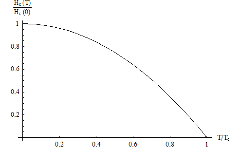
We see that, near $T_{c}$, the dependence of the critical field on temperature does indeed follow the linear relation that we just derived. However, it deviates from said relation when we go far below $T_{c}$. This is not surprising; the GL theory from which we obtained the linear relation is only valid near $T_{c}$. In order to obtain a more accurate relation, we require a theory for the superconductor that is valid far below $T_{c}$.

We may rewrite our dimensionless vector potential and magnetic field in terms of the critical field. We may write our expression for $H_{c}$ as

$H_{c}^{2}=4\pi b\left|\Psi _{0}\right|^{4}.$

Our dimensionless vector potential is then

${\tilde {A}}={\frac {2e}{c}}{\frac {\Psi _{0}}{\sqrt {2mb\Psi _{0}^{4}}}}{\vec {A}}={\frac {2e}{c}}\Psi _{0}{\sqrt {\frac {4\pi }{2mH_{c}^{2}}}}{\vec {A}}={\sqrt {\frac {8\pi e^{2}\Psi _{0}^{2}}{mc^{2}}}}{\vec {A}}={\frac {1}{{\sqrt {2}}H_{c}\lambda }}{\vec {A}}.$

We may rewrite the definition of the magnetic field as

${\vec {B}}={\tilde {\nabla }}\times {\sqrt {2}}H_{c}{\tilde {A}},$

or

${\tilde {\nabla }}\times {\tilde {A}}={\frac {1}{{\sqrt {2}}H_{c}}}{\vec {B}}={\tilde {B}}.$

Magnetic Properties of a Type-I Superconductor

In the approximation stated above, we find that, in the superconducting state (the applied magnetic field is below $H_{c}$), the total magnetic field ${\vec {B}}$ is completely expelled, while ${\vec {B}}={\vec {H}}$ when the applied field is above $H_{c}$. From the defining relation for the magnetization ${\vec {M}}$,

${\vec {B}}={\vec {H}}+4\pi {\vec {M}},$

we find that the magnitude of the magnetization increases linearly with, and points in the opposite direction to, ${\vec {H}}$, in the superconducting state, but is zero in the normal state. We plot these two relations below.

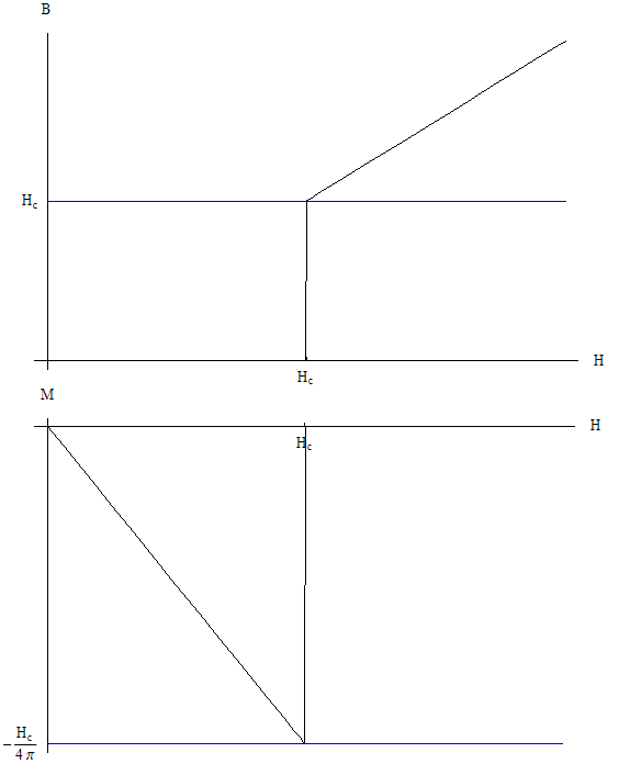
We will now demonstrate two consequences of the total expulsion of a magnetic field from a superconductor.

1) The total field is always tangential to the surface of a superconductor.

First, recall the Maxwell equation,

$\nabla \cdot {\vec {B}}=0.$

Let us now consider the boundary between a superconductor and a normal region:

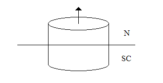
We will find the flux of a magnetic field through the "pill box" shown above. Let the area of the circular surfaces be $\Delta A$, and let us assume that the contribution from the "tube" part of the surface is negligible (we will assume that its height is small compared to the radius of the circular surfaces). Then the total flux may be written as

$B_{n,\bot }\cdot \Delta A-B_{sc,\bot }\cdot \Delta A,$

where $B_{n,\bot }$ and $B_{sc,\bot }$ are the components of the magnetic field normal to the circular surfaces of the "pill box" in the normal and superconducting regions, respectively. The Maxwell equation stated above is equivalent to the statement that the total flux through a closed surface, such as the "pill box" we consider here, must be zero. Therefore,

$B_{n,\bot }=B_{sc,\bot }.$

However, we know that the superconductor completely expels magnetic fields, so that ${\vec {B}}_{sc}=0$. Therefore, $B_{n,\bot }=0$, thus proving that ${\vec {B}}_{n}$ can only have tangential components.

2) As a direct consequence of (1), a type-I superconductor in an external magnetic field always carries an electrical current near its surface.

To show this, first recall the Maxwell equation (Ampere's Law in the case of static fields),

$\nabla \times {\vec {B}}={\frac {4\pi }{c}}{\vec {J}},$

or, in integral form,

$\oint _{\partial S}{\vec {B}}\cdot d{\vec {\ell }}={\frac {4\pi }{c}}I,$

where $S$ is a surface with bounding curve $\partial S$, the line integral on the left is taken in the direction that would cause a right-handed screw to advance in the direction of the normal to the surface, and $I$ is the total current passing through the surface.

Let us now, once again, consider the boundary between a superconductor and a normal region and a rectangular contour drawn around the boundary:

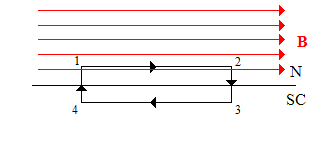
In this case, because the magnetic field is zero in the superconducting region and because the magnetic field in the normal region is tangential to the surface of the superconductor, then, assuming that the lengths of segments 14 and 23 are small compared to that of segments 12 and 34. In this case, the left-hand side of the Maxwell equation becomes

$\oint _{\partial S}{\vec {B}}\cdot d{\vec {\ell }}=B\ell _{12},$

where $\ell _{12}$ is the length of segment 12. The right-hand side, on the other hand, is

${\frac {4\pi }{c}}I={\frac {4\pi }{c}}K\ell _{12},$

where $K$ is the surface current density (per unit length). This implies that

$B={\frac {4\pi }{c}}K,$

or, in vector form,

${\vec {K}}={\frac {c}{4\pi }}{\hat {n}}\times {\vec {B}},$

where ${\hat {n}}$ is the normal to the surface pointing into the normal region. In this case, we see that ${\vec {K}}$ points into the page or screen.

An Example: The Magnetic Field Around a Spherical Superconductor

These observations lead to interesting conclusions for superconductors with geometries more complex than a cylinder inside a magnetic field parallel to its axis. Consider, for example, a spherical superconductor, depicted below:

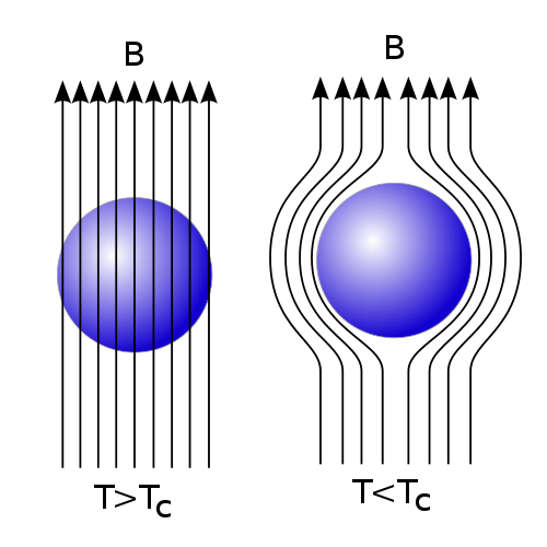
As we can see, the magnetic field near the equator is stronger than the applied field, while the field at the poles vanishes. This implies that the magnetic field near the equator may exceed $H_{c}$ even if the applied field is less than $H_{c}$, simply due to the geometry of the sample. In fact, for a certain range of fields,

$(1-\eta )H_{c}<H<H_{c},$

the sample will enter an intermediate state, in which superconducting and normal regions coexist. The above inequality holds for any geometry, in fact, and $\eta$ is known as the demagnetizing factor of the sample. Its value will depend on the exact geometry of the sample; we will now show that, for a sphere, $\eta ={\tfrac {1}{3}}$. We will do so by solving Maxwell's equations for a spherical superconductor of radius $R$ in a uniform applied magnetic field ${\vec {H}}=H{\hat {z}}$. The boundary conditions for this problem are

${\vec {B}}({\vec {r}})=H{\hat {z}}$

for $|{\vec {r}}|\rightarrow \infty$ and

${\hat {n}}\cdot {\vec {B}}({\vec {r}})=0$

on the surface of the sphere. Outside the superconductor, the equations satisfied by ${\vec {B}}$ are

$\nabla \cdot {\vec {B}}=0$

and

$\nabla \times {\vec {B}}=0.$

The second equation implies that there are no current sources outside the superconductor. It also implies that we may write the magnetic field in terms of a scalar potential. We therefore write

${\vec {B}}=\nabla \Phi +H{\vec {z}}.$

Substituting this into the first equation, we get

$\nabla ^{2}\Phi =0,$

which is just Laplace's equation. Our boundary conditions for $\Phi$ are, in spherical coordinates,

$\Phi ({\vec {r}}\rightarrow \infty )=0$

and

${\frac {\partial \Phi }{\partial r}}+H\cos {\theta }=0$

on the surface. Laplace's equation in spherical coordinates is

${\frac {1}{r^{2}}}{\frac {\partial }{\partial r}}\left(r^{2}{\frac {\partial \Phi }{\partial r}}\right)+{\frac {1}{r^{2}\sin {\theta }}}{\frac {\partial }{\partial \theta }}\left(\sin {\theta }{\frac {\partial \Phi }{\partial \theta }}\right)+{\frac {1}{r^{2}\sin ^{2}{\theta }}}{\frac {\partial ^{2}\Phi }{\partial \phi ^{2}}}=0.$

Because our system has azimuthal symmetry, $\Phi$ should be independent of $\phi$. Therefore, $\Phi ({\vec {r}})=\Phi (r,\theta )$ and Laplace's equation becomes

${\frac {1}{r^{2}}}{\frac {\partial }{\partial r}}\left(r^{2}{\frac {\partial \Phi }{\partial r}}\right)+{\frac {1}{r^{2}\sin {\theta }}}{\frac {\partial }{\partial \theta }}\left(\sin {\theta }{\frac {\partial \Phi }{\partial \theta }}\right)=0.$

Multiplying by $r^{2}$, we get

${\frac {\partial }{\partial r}}\left(r^{2}{\frac {\partial \Phi }{\partial r}}\right)+{\frac {1}{\sin {\theta }}}{\frac {\partial }{\partial \theta }}\left(\sin {\theta }{\frac {\partial \Phi }{\partial \theta }}\right)=0.$

We will now attempt to solve this equation by separation of variables. Let us try a solution of the form

$\Phi (r,\theta )=R(r)\chi (\theta ).$

Then

${\frac {1}{R}}{\frac {d}{dr}}\left(r^{2}{\frac {dR}{dr}}\right)=-{\frac {1}{\chi }}{\frac {1}{\sin {\theta }}}{\frac {d}{d\theta }}\left(\sin {\theta }{\frac {d\chi }{d\theta }}\right).$

We see that we have an expression depending only on $r$ on one side and one depending only on $\theta$ on the other. The only way for this equation to be satisfied is if both equal a constant, which we will call $-\lambda$. Let us first consider the equation for $\chi$. This equation is

${\frac {1}{\sin {\theta }}}{\frac {d}{d\theta }}\left(\sin {\theta }{\frac {d\chi }{d\theta }}\right)=\lambda \chi .$

If we make the substitution, $x=\cos {\theta }$, into this equation, we get

${\frac {d}{dx}}\left[(1-x^{2}){\frac {d\chi }{dx}}\right]=\lambda \chi .$

We recognize this as the Legendre differential equation. The only physically interesting solutions to this equation occur when $\lambda =-l(l+1)$, in which case we find that $\chi$ is a Legendre polynomial,

$\chi (\theta )=P_{l}(\cos {\theta }).$

The first few Legendre polynomials are $P_{0}(x)=1$, $P_{1}(x)=x$, and $P_{2}(x)={\tfrac {1}{2}}(3x^{2}-1)$.

Now we will consider the equation for $R$. If we take $\chi (\theta )=P_{l}(\cos {\theta })$, then our differential equation for $R$ becomes

${\frac {d}{dr}}\left(r^{2}{\frac {dR}{dr}}\right)=l(l+1)R,$

or

${\frac {d^{2}R}{dr^{2}}}+2r{\frac {dR}{dr}}-l(l+1)R=0.$

This is an Euler-Cauchy differential equation. Let us assume a power law dependence for $R$,

$R(r)=r^{\alpha }.$

The equation becomes

$\alpha (\alpha -1)r^{\alpha }+2\alpha r^{\alpha }-l(l+1)r^{\alpha }=0.$

The exponent $\alpha$ must therefore satisfy

$\alpha (\alpha +1)=l(l+1).$

This equation has two possible solutions, $\alpha =l$ and $\alpha =-(l+1)$, so the general solution for the differential equation is

$R(r)=A_{l}r^{l}+{\frac {B_{l}}{r^{l+1}}}.$

The general solution to the original partial differential equation is then a linear combination of all possible products $R(r)\chi (\theta )$,

$\Phi (r,\theta )=\sum _{l=0}^{\infty }\left(A_{l}r^{l}+{\frac {B_{l}}{r^{l+1}}}\right)P_{l}(\cos {\theta }).$

Since $r^{l}\rightarrow \infty$ for all $l>0$, we must set $A_{l}=0$ for all such values of $l$. We will also set $A_{0}=0$, so that

$\Phi (r,\theta )=\sum _{l=0}^{\infty }{\frac {B_{l}}{r^{l+1}}}P_{l}(\cos {\theta }).$

We now apply the boundary condition,

${\frac {\partial \Phi }{\partial r}}+H\cos {\theta }=0,$

to obtain

$\sum _{l=0}^{\infty }{\frac {(l+1)B_{l}}{R^{l+2}}}P_{l}(\cos {\theta })=H\cos {\theta }.$

By inspection, we find that $B_{l}=0$ for all $l\neq 1$. For $l=1$, we have

$B_{l}={\tfrac {1}{2}}HR^{3}.$

Therefore, the solution for $\Phi$ is

$\Phi (r,\theta )={\frac {HR^{3}}{2r^{2}}}\cos {\theta },$

and thus ${\vec {B}}$ is

${\vec {B}}={\tfrac {1}{2}}HR^{3}\nabla \left({\frac {\cos {\theta }}{r^{2}}}\right)+H{\hat {z}}.$

In spherical coordinates, the gradient operator is given by

$\nabla \Phi ={\frac {\partial \Phi }{\partial r}}{\hat {r}}+{\frac {1}{r}}{\frac {\partial \Phi }{\partial \theta }}{\hat {\theta }}+{\frac {1}{r\sin {\theta }}}{\frac {\partial \Phi }{\partial \phi }}{\hat {\phi }},$

so

${\vec {B}}=-H\left({\frac {R}{r}}\right)^{3}(\cos {\theta }{\hat {r}}+{\tfrac {1}{2}}\sin {\theta }{\hat {\theta }})+H{\hat {z}}.$

We recognize that ${\hat {z}}=\cos {\theta }{\hat {r}}-\sin {\theta }{\hat {\theta }}$, so that

${\vec {B}}=\left[1-\left({\frac {R}{r}}\right)^{3}\right]H\cos {\theta }{\hat {r}}-\left[1+{\tfrac {1}{2}}\left({\frac {R}{r}}\right)^{3}\right]H\sin {\theta }{\hat {\theta }}.$

We now want to find the point at which the magnetic field has the largest magnitude. The magnitude of this vector is given by

$|{\vec {B}}|^{2}=H^{2}\left[1+{\tfrac {1}{2}}\left({\frac {R}{r}}\right)^{3}\right]^{2}+3\left({\frac {R}{r}}\right)^{3}\left[{\tfrac {1}{4}}\left({\frac {R}{r}}\right)^{3}-1\right]\cos ^{2}{\theta }$

We see that the second term, which is proportional to $\cos ^{2}{\theta }$, is clearly negative when $r>R$. Therefore, we must make the size of this term as small as possible. This may be done by letting $\theta ={\tfrac {\pi }{2}}$. For this value of $\theta$, we have

$|{\vec {B}}|^{2}=H^{2}\left[1+{\tfrac {1}{2}}\left({\frac {R}{r}}\right)^{3}\right]^{2}.$

This function is monotonically decreasing as we increase $r$; therefore, we choose the smallest possible value of $r$, which is $r=R$. This gives us

$|{\vec {B}}|^{2}={\tfrac {9}{4}}H^{2},$

or $|{\vec {B}}|={\tfrac {3}{2}}H$. Therefore, the total magnetic field achieves its maximum magnitude at the equator of the sphere, where it is three halves the applied field. Therefore, if the applied field is larger than $H={\tfrac {2}{3}}H_{c}$, the field at the equator would become larger than $H_{c}$, which would destroy the sphere's superconductivity at that point. Therefore, the sphere enters an intermediate state when ${\tfrac {2}{3}}H_{c}<H<H_{c}$, so that the demagnetizing factor $\eta ={\tfrac {1}{3}}$.

Superconductors of General Geometries

In general, the maximum magnetic field on the surface of a superconductor will be related to the applied field by

$B_{\text{max}}={\frac {H}{1-\eta }}.$

We will now list the values of $\eta$ for a few different geometries.

Geometry	Demagnetizing factor $\eta$
Cylinder with ${\vec {H}}$ parallel to its axis	$0$
Cylinder with ${\vec {H}}$ perpendicular to its axis	${\tfrac {1}{2}}$
Sphere	${\tfrac {1}{3}}$
Infinite thin plate with ${\vec {H}}$ perpendicular to the plate	$1$

The sample will enter the intermediate state at the value of $H=H^{\ast }$ at which $B_{\text{max}}=H_{c}$, which is

$H^{\ast }=(1-\eta )H_{c}.$

Therefore, the superconductor will be in the intermediate state when

$(1-\eta )H_{c}<H<H_{c}.$

We will now show plots of the magnetic field of a sphere at the equator and at the pole as a function of the applied field (for details on how to derive the dependence in the intermediate state, see P. G. DeGennes, Superconductivity of Metals and Alloys).

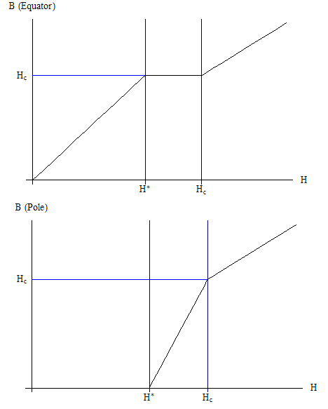
In the intermediate state, the energy per volume of both the normal and superconducting states is the same. Therefore, the energy per unit area of a "domain wall" will be the dominant contribution.

Surface Term of the Free Energy

The free energy in the reduced units can be written as

$F=\int d^{3}r\,\left[\alpha (T-T_{c})|\Psi |^{2}+{\frac {b}{2}}|\Psi |^{4}+{\frac {\hbar ^{2}}{2m}}|(\nabla -{\frac {2ei}{\hbar c}}{\vec {A}})\Psi |^{2}+{\frac {1}{8\pi }}(\nabla \times {\vec {A}})^{2}-{\frac {1}{4\pi }}{\vec {H}}\cdot {\vec {B}}\right]$

$=\lambda ^{D}\int d^{D}{\tilde {r}}\,\left[\alpha (T-T_{c})|\Psi _{o}|^{2}|\psi |^{2}+{\frac {b}{2}}|\Psi _{o}|^{4}|\psi |^{4}+{\frac {\hbar ^{2}}{2m_{GL}}}|\Psi _{o}|^{2}|({\frac {1}{\lambda }}{\tilde {\nabla }}-{\frac {2ei}{\hbar c}}{\sqrt {2}}\lambda H_{c}{\tilde {A}})\psi |^{2}+{\frac {1}{8\pi \lambda ^{2}}}({\sqrt {2}}\lambda H_{c})^{2}({\tilde {\nabla }}\times {\tilde {A}})^{2}-{\frac {2\lambda ^{2}H_{c}^{2}}{4\pi \lambda ^{2}}}{\tilde {H}}\cdot {\tilde {B}}\,\right]$

where

${\tilde {r}}={\frac {r}{\lambda }},{\tilde {H}}={\frac {H}{{\sqrt {2}}H_{c}}}$

Using the following relations:

$b|\Psi _{o}|^{4}={\frac {H_{c}^{2}}{4\pi }}$

${\frac {\alpha (T-T_{c})}{b|\Psi _{o}|^{2}}}=-1$

$|\Psi _{o}|^{2}{\frac {4e^{2}}{mc^{2}}}={\frac {1}{4\pi \lambda ^{2}}}$

one has

$F={\frac {\lambda ^{D}H_{c}^{2}}{4\pi }}\int d^{D}{\tilde {r}}\,\left[-|\psi |^{2}+{\frac {1}{2}}|\psi |^{4}+|({\frac {1}{\kappa }}{\frac {\tilde {\nabla }}{i}}-{\tilde {A}})\psi |^{2}+{\tilde {B}}^{2}-2{\tilde {H}}\cdot {\tilde {B}}\,\right]$

Now let's consider the gradinet term:

$|({\frac {1}{\kappa }}{\frac {\tilde {\nabla }}{i}}-{\tilde {A}})\psi |^{2}=\,\left[({\frac {-1}{\kappa }}{\frac {\tilde {\nabla }}{i}}-{\tilde {A}})\psi ^{*}\,\right]\,\left[({\frac {1}{\kappa }}{\frac {\tilde {\nabla }}{i}}-{\tilde {A}})\psi \,\right]=(-{\tilde {A}}\psi ^{*})({\frac {1}{\kappa }}{\frac {\tilde {\nabla }}{i}}-{\tilde {A}})\psi -({\frac {1}{\kappa }}{\frac {\tilde {\nabla }}{i}}\psi ^{*})({\frac {1}{\kappa }}{\frac {\tilde {\nabla }}{i}}-{\tilde {A}})\psi$

Integration by part leads the 2nd term to the form:

$-{\tilde {\nabla }}\cdot ({\frac {1}{\kappa }}{\frac {1}{i}}\psi ^{*}({\frac {1}{\kappa }}{\frac {\tilde {\nabla }}{i}}-{\tilde {A}})\psi )+\psi ^{*}({\frac {1}{\kappa }}{\frac {\tilde {\nabla }}{i}}({\frac {1}{\kappa }}{\frac {\tilde {\nabla }}{i}}-{\tilde {A}})\psi )$

where the 1st term needs to be evaluated on the surface where it vanishes by the boundary condition for an insulating interface. Hence the gradient term becomes

$|({\frac {1}{\kappa }}{\frac {\tilde {\nabla }}{i}}-{\tilde {A}})\psi |^{2}=\psi ^{*}({\frac {1}{\kappa }}{\frac {\tilde {\nabla }}{i}}-{\tilde {A}})^{2}\psi$

Assuming that $\psi$ and ${\tilde {A}}$ satisfy the GL equation, namely,

$({\frac {1}{\kappa }}{\frac {\tilde {\nabla }}{i}}-{\tilde {A}})^{2}\psi =\psi -\psi |\psi |^{2}$

we have

$\psi ^{*}({\frac {1}{\kappa }}{\frac {\tilde {\nabla }}{i}}-{\tilde {A}})^{2}\psi =|\psi |^{2}-|\psi |^{4}$

and the free energy becomes

$F={\frac {\lambda ^{D}H_{c}^{2}}{4\pi }}\int d^{D}{\tilde {r}}\,\left[-{\frac {1}{2}}|\psi |^{4}+{\tilde {B}}^{2}-2{\tilde {H}}\cdot {\tilde {B}}\,\right]$

This is true at the saddle point. Now the free energy for the normal state and the superconducting state are given by

$F_{n}={\frac {\lambda ^{D}H_{c}^{2}}{4\pi }}\int d^{D}{\tilde {r}}\,\left[-{\tilde {H}}^{2}\,\right]$

and

$F_{s}={\frac {\lambda ^{D}H_{c}^{2}}{4\pi }}\int d^{D}{\tilde {r}}\,\left[-{\frac {1}{2}}|\psi |^{4}+{\tilde {B}}^{2}-2{\tilde {B}}\cdot {\tilde {H}}\,\right]$

Therefore, the surface free energy of the interface is

$F_{s}-F_{n}={\frac {\lambda ^{D}H_{c}^{2}}{4\pi }}\int d^{D}{\tilde {r}}\,\left[-{\frac {1}{2}}|\psi |^{4}+{\tilde {B}}^{2}-2{\tilde {B}}\cdot {\tilde {H}}+{\tilde {H}}^{2}\,\right]={\frac {\lambda ^{D}H_{c}^{2}}{4\pi }}\int d^{D}{\tilde {r}}\,\left[-{\frac {1}{2}}|\psi |^{4}+({\tilde {B}}-{\tilde {H}})^{2}\,\right]$

Free Energy of a Normal-Superconducting Interface

Now let's consider the free energy of a normal-superconducting interface. Recall the GL equations:

$({\frac {1}{\kappa }}{\frac {\tilde {\nabla }}{i}}-{\tilde {A}})^{2}\psi -\psi +\psi |\psi |^{2}=0$

${\frac {1}{2}}(\psi ^{*}{\frac {1}{\kappa }}{\frac {\tilde {\nabla }}{i}}\psi +c.c.)-{\tilde {A}}|\psi |^{4}={\tilde {\nabla }}\times ({\tilde {\nabla }}\times {\tilde {A}})$

Assume that the interface is along y-z plane and ${\tilde {B}}//{\hat {z}}$. We can choose ${\tilde {A}}({\tilde {r}})={\hat {y}}{\tilde {A}}({\tilde {x}})$ which implies the order parameter depends only on ${\tilde {x}}$. Then the GL equation become

$-{\frac {1}{\kappa ^{2}}}{\frac {d^{2}\psi }{d{\tilde {x}}^{2}}}+{\tilde {A}}_{y}^{2}({\tilde {x}})\psi -\psi +\psi ^{3}=0$(*)

${\tilde {A}}_{y}({\tilde {x}})\psi ^{2}={\frac {d^{2}{\tilde {A}}_{y}({\tilde {x}})}{d{\tilde {x}}^{2}}}$

and

${\frac {1}{2}}(\psi ^{*}{\frac {1}{\kappa }}{\frac {1}{i}}{\frac {d}{d{\tilde {x}}}}\psi +c.c.)=0$

Note that we can choose $\psi$ to be real since the coefficients are real. Now let's manipulate Eq.(*):

$-{\frac {1}{\kappa ^{2}}}{\frac {d\psi }{d{\tilde {x}}}}{\frac {d^{2}\psi }{d{\tilde {x}}^{2}}}+{\tilde {A}}_{y}^{2}{\frac {d\psi }{d{\tilde {x}}}}\psi -{\frac {d\psi }{d{\tilde {x}}}}\psi +{\frac {d\psi }{d{\tilde {x}}}}\psi ^{3}=0$

$-{\frac {1}{2\kappa ^{2}}}{\frac {d}{d{\tilde {x}}}}({\frac {d\psi }{d{\tilde {x}}}})^{2}+{\frac {1}{2}}{\tilde {A}}_{y}^{2}{\frac {d}{d{\tilde {x}}}}\psi ^{2}-{\frac {1}{2}}{\frac {d}{d{\tilde {x}}}}\psi ^{2}+{\frac {1}{4}}{\frac {d}{\tilde {x}}}\psi ^{4}=0$

Integrating we have

$-{\frac {1}{2\kappa ^{2}}}({\frac {d\psi }{d{\tilde {x}}}})^{2}+{\frac {1}{2}}\int d{\tilde {x}}{\tilde {A}}_{y}^{2}{\frac {d}{d{\tilde {x}}}}\psi ^{2}-{\frac {1}{2}}\psi ^{2}+{\frac {1}{4}}\psi ^{4}=const.$

This integral can be further manipulated:

$\int d{\tilde {x}}{\tilde {A}}_{y}^{2}{\frac {d}{d{\tilde {x}}}}\psi ^{2}=\int d{\tilde {x}}\,\left[{\frac {d}{d{\tilde {x}}}}({\tilde {A}}_{y}^{2}\psi ^{2})-{\frac {d{\tilde {A}}_{y}^{2}}{d{\tilde {x}}}}\psi ^{2}\,\right]={\tilde {A}}_{y}^{2}\psi ^{2}-2\int d{\tilde {x}}{\tilde {A}}_{y}{\frac {d{\tilde {A}}_{y}}{d{\tilde {x}}}}\psi ^{2}={\tilde {A}}_{y}^{2}\psi ^{2}-2\int d{\tilde {x}}{\frac {d{\tilde {A}}_{y}}{d{\tilde {x}}}}{\frac {d^{2}{\tilde {A}}_{y}}{d{\tilde {x}}^{2}}}={\tilde {A}}_{y}^{2}\psi ^{2}-\int d{\tilde {x}}{\frac {d}{d{\tilde {x}}}}({\frac {d{\tilde {A}}_{y}}{d{\tilde {x}}}})^{2}={\tilde {A}}_{y}^{2}\psi ^{2}-({\frac {d{\tilde {A}}_{y}}{d{\tilde {x}}}})^{2}=const.$

Thus, Eq.(*) becomes

$-{\frac {1}{2\kappa ^{2}}}({\frac {d\psi }{d{\tilde {x}}}})^{2}+{\frac {1}{2}}{\tilde {A}}_{y}^{2}\psi ^{2}-{\frac {1}{2}}({\frac {d{\tilde {A}}_{y}}{d{\tilde {x}}}})^{2}-{\frac {1}{2}}\psi ^{2}+{\frac {1}{4}}\psi ^{4}=const.$

or,

${\frac {1}{\kappa ^{2}}}({\frac {d\psi }{d{\tilde {x}}}})^{2}+({\frac {d{\tilde {A}}_{y}}{d{\tilde {x}}}})^{2}+\psi ^{2}(1-{\tilde {A}}_{y}^{2})-{\frac {1}{2}}\psi ^{4}=const.$

To determine the const., note that as $x\rightarrow -\infty$, $\psi \rightarrow 1$ and ${\tilde {A}}_{y}\rightarrow 0$, so

$0+0+1-{\frac {1}{2}}=const.$

Therefore,

${\frac {1}{\kappa ^{2}}}({\frac {d\psi }{d{\tilde {x}}}})^{2}+({\frac {d{\tilde {A}}_{y}}{d{\tilde {x}}}})^{2}+\psi ^{2}(1-{\tilde {A}}_{y}^{2})-{\frac {1}{2}}\psi ^{4}={\frac {1}{2}}$

Consider the case where $\kappa <<1$, that is, $\lambda <<\xi$. The main contribution to the surface energy comes from the region where ${\tilde {B}}=0$ but $\psi <1$.

${\frac {1}{\kappa ^{2}}}({\frac {d\psi }{d{\tilde {x}}}})^{2}+\psi ^{2}-{\frac {1}{2}}\psi ^{4}={\frac {1}{2}}$

${\frac {1}{\kappa ^{2}}}({\frac {d\psi }{d{\tilde {x}}}})^{2}={\frac {1}{2}}-\psi ^{2}+{\frac {1}{2}}\psi ^{4}={\frac {1}{2}}(1-\psi ^{2})^{2}$

${\frac {1}{\kappa }}{\frac {d\psi }{d{\tilde {x}}}}=-{\frac {1}{\sqrt {2}}}(1-\psi ^{2})$

Note that the minus sign is from the experimental setup. Further,

${\frac {d\psi }{1-\psi ^{2}}}=-{\frac {\kappa }{\sqrt {2}}}d{\tilde {x}};{\frac {1}{1-\psi ^{2}}}={\frac {1}{2}}({\frac {1}{1-\psi }}+{\frac {1}{1+\psi }})$

$ln{\frac {1+\psi }{1-\psi }}=-{\sqrt {2}}\kappa {\tilde {x}}+const.$

${\frac {1+\psi ({\tilde {x}})}{1-\psi ({\tilde {x}})}}=const.\times e^{-{\sqrt {2}}\kappa {\tilde {x}}}$

Requiring $\psi =0$ at ${\tilde {x}}=0$ gives $const.=1$ Now we have

$\psi ={\frac {e^{-{\sqrt {2}}\kappa {\tilde {x}}}-1}{e^{-{\sqrt {2}}\kappa {\tilde {x}}}+1}}=-tanh{\frac {\kappa {\tilde {x}}}{\sqrt {2}}}$

Moreover,

$F_{s}-F_{n}={\frac {H_{c}^{2}}{8\pi }}L^{2}\lambda \int _{-\infty }^{0}d{\tilde {x}}(1-\psi ^{4})$

where

$\int _{-\infty }^{0}d{\tilde {x}}(1-\psi ^{4})=\int _{-\infty }^{0}d{\tilde {x}}(1+\psi ^{2})(1-\psi ^{2})=\int _{-\infty }^{0}d{\tilde {x}}(1+\psi ^{2})(-{\frac {\sqrt {2}}{\kappa }}){\frac {d\psi }{d{\tilde {x}}}}=-{\frac {\sqrt {2}}{\kappa }}\psi |_{-\infty }^{0}-{\frac {\sqrt {2}}{\kappa }}\int _{-\infty }^{0}d{\tilde {x}}\psi ^{2}{\frac {d\psi }{d{\tilde {x}}}}$

$=-{\frac {\sqrt {2}}{\kappa }}\psi |_{-\infty }^{0}-{\frac {\sqrt {2}}{3\kappa }}\int _{-\infty }^{0}d{\tilde {x}}{\frac {d\psi ^{3}}{d{\tilde {x}}}}=-{\frac {\sqrt {2}}{\kappa }}\psi |_{-\infty }^{0}-{\frac {\sqrt {2}}{3\kappa }}\psi ^{3}|_{-\infty }^{0}={\frac {\sqrt {2}}{\kappa }}+{\frac {\sqrt {2}}{3\kappa }}={\frac {4{\sqrt {2}}}{3\kappa }}$

Hence one has

$F_{s}-F_{n}={\frac {H_{c}^{2}}{8\pi }}L^{2}\lambda \cdot {\frac {4{\sqrt {2}}}{3\kappa }}$

Below we show that given $\psi$ and ${\tilde {A}}_{y}$ satisfying the GL equation, the surface energy of the surface vanishes at $\kappa =1/2$:

${\frac {1}{\kappa ^{2}}}({\frac {d\psi }{d{\tilde {x}}}})^{2}+({\frac {d{\tilde {A}}_{y}}{d{\tilde {x}}}})^{2}+\psi ^{2}(1-{\tilde {A}}_{y}^{2})-{\frac {1}{2}}\psi ^{4}={\frac {1}{2}}$(**)

$F_{s}-F_{n}={\frac {H_{c}^{2}}{4\pi }}L^{2}\lambda \int d{\tilde {x}}\,\left[({\tilde {B}}-{\tilde {H}})^{2}-{\frac {1}{2}}\psi ^{4}\,\right]$

Assume $\kappa =1/{\sqrt {2}}$.

$F_{s}-F_{n}={\frac {H_{c}^{2}}{4\pi }}L^{2}\lambda \int d{\tilde {x}}\,\left[({\frac {d{\tilde {A}}_{y}}{d{\tilde {x}}}}-{\frac {1}{\sqrt {2}}})^{2}-{\frac {1}{2}}\psi ^{4}\,\right]$

Choosing

${\frac {d{\tilde {A}}_{y}}{d{\tilde {x}}}}={\frac {1}{\sqrt {2}}}-{\frac {1}{\sqrt {2}}}\psi ^{2}$

then $F_{s}-F_{n}=0$ and the 2nd GL equation becomes

${\tilde {A}}_{y}\psi ^{2}={\frac {d^{2}{\tilde {A}}_{y}}{d{\tilde {x}}^{2}}}={\frac {d}{d{\tilde {x}}}}({\frac {1}{\sqrt {2}}}-{\frac {1}{\sqrt {2}}}\psi ^{2})=-{\sqrt {2}}\psi {\frac {d\psi }{d{\tilde {x}}}}$

${\frac {d\psi }{d{\tilde {x}}}}=-{\frac {1}{\sqrt {2}}}{\tilde {A}}_{y}\psi$

Insert this into Eq.(**):

${\frac {1}{\kappa ^{2}}}{\frac {1}{2}}{\tilde {A}}_{y}^{2}\psi ^{2}+({\frac {1}{\sqrt {2}}}-{\frac {1}{\sqrt {2}}}\psi ^{2})^{2}+\psi ^{2}(1-{\tilde {A}}_{y}^{2})-{\frac {1}{2}}\psi ^{4}-{\frac {1}{2}}=0$

${\frac {1}{2\kappa ^{2}}}{\tilde {A}}_{y}^{2}\psi ^{2}+{\frac {1}{2}}-\psi ^{2}+{\frac {1}{2}}\psi ^{4}+\psi ^{2}-{\tilde {A}}_{y}^{2}\psi ^{2}-{\frac {1}{2}}\psi ^{4}-{\frac {1}{2}}=0$

$({\frac {1}{2\kappa ^{2}}}-1){\tilde {A}}_{y}^{2}\psi ^{2}=0$

Therefore, $\kappa =1/{\sqrt {2}}$ as expected.

In summary, for type-I superconductor (positive surface energy) $\kappa <1/{\sqrt {2}}$ and $\psi$ is uniform in the bulk and jumps at $T_{c}$. On the other hand, for type-II superconductor (negative surface energy) $\kappa >1/{\sqrt {2}}$ and $\psi$ is not uniform in the bulk but grows continuously when crossing $T_{c}$ from above.

The "Landau-Level"-Like States above Hc and the upper critical field Hc2

Now we have the surface free energy:

$F_{s}-F_{n}={\frac {H_{c}^{2}}{4\pi }}\lambda ^{3}\int d^{3}{\tilde {r}}\,\left[-|\psi |^{2}+|({\frac {1}{\kappa }}{\frac {\tilde {\nabla }}{i}}-{\tilde {A}})^{2}\psi |^{2}+{\frac {1}{2}}|\psi |^{4}+({\tilde {B}}-{\tilde {H}})^{2}\,\right]$

where

${\tilde {B}}={\frac {B}{{\sqrt {2}}H_{c}}}$ and ${\tilde {A}}={\frac {A}{{\sqrt {2}}\lambda H_{c}}}$

Assuming 2nd order phase transition and $T=T_{c}$, then $\psi \rightarrow 0$ and ${\tilde {B}}\rightarrow {\tilde {H}}$:

$F_{s}-F_{n}={\frac {H_{c}^{2}}{4\pi }}\lambda ^{3}\int d^{3}{\tilde {r}}\,\left[-|\psi |^{2}+|({\frac {1}{\kappa }}{\frac {\tilde {\nabla }}{i}}-{\tilde {A}})^{2}\psi |^{2}\,\right]$

Using the Landau gauge:

${\vec {A}}={\hat {y}}Hx={\hat {y}}{\frac {H}{{\sqrt {2}}H_{c}}}{\frac {x}{\lambda }}={\hat {y}}{\tilde {H}}{\tilde {x}}$

Recall

$({\frac {1}{\kappa }}{\frac {\tilde {\nabla }}{i}}-{\tilde {A}})^{2}\psi -\psi =0$

$({\frac {1}{\kappa }}{\frac {1}{i}}{\frac {d}{d{\tilde {x}}}})^{2}\psi +({\frac {1}{\kappa }}{\frac {1}{i}}{\frac {d}{d{\tilde {y}}}}-{\tilde {H}}{\tilde {x}})^{2}\psi +({\frac {1}{\kappa }}{\frac {1}{i}}{\frac {d}{d{\tilde {z}}}})^{2}\psi -\psi =0$

$-{\frac {1}{\kappa ^{2}}}{\frac {d^{2}}{d{\tilde {x}}^{2}}}\psi +({\frac {1}{\kappa }}{\frac {1}{i}}{\frac {d}{d{\tilde {y}}}}-{\tilde {H}}{\tilde {x}})^{2}\psi -{\frac {1}{\kappa ^{2}}}{\frac {d^{2}}{d{\tilde {z}}^{2}}}\psi -\psi =0$

Let

$\psi ({\tilde {x}},{\tilde {y}},{\tilde {z}})=e^{ik_{z}{\tilde {z}}}e^{ik{\tilde {y}}}\Phi _{k}({\tilde {x}})$

then

$e^{ik_{z}{\tilde {z}}}e^{ik{\tilde {y}}}\,\left[-{\frac {1}{\kappa ^{2}}}{\frac {d^{2}}{d{\tilde {x}}^{2}}}\Phi +({\frac {k}{\kappa }}-{\tilde {H}}{\tilde {x}})^{2}\Phi +{\frac {k_{z}^{2}}{\kappa ^{2}}}\Phi -\Phi \,\right]=0$

Let

$-{\tilde {H}}X={\frac {k}{\kappa }}-{\tilde {H}}{\tilde {x}};{\frac {d}{d{\tilde {x}}}}={\frac {dX}{d{\tilde {x}}}}{\frac {d}{dX}}={\frac {d}{dX}}$

then

$e^{ik_{z}{\tilde {z}}}e^{ik{\tilde {y}}}(-{\frac {1}{\kappa ^{2}}}{\frac {d^{2}}{dX^{2}}}+{\tilde {H}}^{2}X^{2}+{\frac {k_{z}^{2}}{\kappa ^{2}}}-1)\Phi =0$

Recall for a harmonic oscillator we have

$({\frac {-\hbar ^{2}}{2m}}{\frac {d^{2}}{dx^{2}}}+{\frac {1}{2}}m\omega ^{2}x^{2})\Psi =E\Psi$

and

$E=\hbar \omega (n+{\frac {1}{2}})$

Comparison leads to

${\frac {-\hbar ^{2}}{2m}}\rightarrow {\frac {-1}{\kappa ^{2}}};{\frac {1}{2}}m\omega ^{2}\rightarrow {\tilde {H}}^{2};\hbar \omega \rightarrow {\frac {2{\tilde {H}}}{\kappa }}$

and the eigenvalues

$2{\frac {\tilde {H}}{\kappa }}(n+{\frac {1}{2}})+{\frac {k_{z}}{\kappa }}-1$

The exponent is zero when

$2{\frac {\tilde {H}}{\kappa }}(n+{\frac {1}{2}})+{\frac {k_{z}}{\kappa }}-1=0$

If $n=0$ and $k_{x}=0$ we have

${\tilde {H}}_{c2}=\kappa ={\frac {H_{c2}}{{\sqrt {2}}H_{c}}}$

$H_{c2}={\sqrt {2}}\kappa H_{c}$

For $\kappa <1/{\sqrt {2}}$, $H_{c2}<H_{c}$, the bulk is preempted by the Meissner phase. On the other hand, $\kappa >1/{\sqrt {2}}$, $H_{c2}>H_{c}$, the bulk undergoes a 2nd order phase transition into a mixed state in which normal state and superconducting state coexist.

Now let's look at the wavefunction at $H_{c2}$.

$(-{\frac {1}{\kappa ^{2}}}{\frac {d^{2}}{dX^{2}}}+{\tilde {H}}_{c2}^{2}X^{2})\Phi =\lambda \Phi ;{\tilde {H}}_{c2}=\kappa$

$(-{\frac {1}{\kappa ^{2}}}{\frac {d^{2}}{dX^{2}}}+\kappa ^{2}X^{2})\Phi =\lambda \Phi$

Let

${\frac {1}{\sqrt {2}}}{\frac {1}{\kappa }}{\frac {d}{dX}}+{\frac {1}{\sqrt {2}}}\kappa X=a$

${\frac {-1}{\sqrt {2}}}{\frac {1}{\kappa }}{\frac {d}{dX}}+{\frac {1}{\sqrt {2}}}\kappa X=a^{+}$

where $[a,a^{+}]=1$ Note that

$a^{+}a={\frac {-1}{2\kappa ^{2}}}{\frac {d^{2}}{dX^{2}}}+{\frac {1}{2}}\kappa ^{2}X^{2}-{\frac {1}{2}}$

$(2a^{+}a+1)\Phi =\lambda \Phi$

For $\lambda =1$ we have

${\frac {1}{\sqrt {2}}}({\frac {1}{\kappa }}{\frac {d}{dX}}+\kappa K)\Phi =0$

$\Phi =const.\times e^{-{\frac {1}{2}}\kappa ^{2}X^{2}}$

and the order parameter is of the form

$const.\times e^{ik{\tilde {y}}}e^{-{\frac {\kappa ^{2}}{2}}({\tilde {x}}-{\frac {k}{\kappa ^{2}}})^{2}}$

Abrikosov Solution of the GL Equation for Type-II Superconductor near Hc2

Note. In this section we will drop the "tilde(~)" on relevant quantities and recover it when necessary.

Since the conditions along the entire superconductor are uniform, we seek a linear combination of solutions centered through equal intervals, namely,

$\psi ^{(0)}=\Sigma _{n=-\infty }^{\infty }C_{n}e^{ikn{\hat {y}}}e^{-{\frac {1}{2}}\kappa ^{2}(x-{\frac {kn}{\kappa ^{2}}})^{2}}$

or,

$\psi =\Sigma _{n=-\infty }^{\infty }C_{n}e^{ikny}\phi _{n}(x)$

with

$\phi _{n}(x)=e^{-{\frac {1}{2}}\kappa ^{2}(x-{\frac {kn}{\kappa ^{2}}})^{2}}$

Consider the solution to GL equation at $H$ slightly less than $\kappa$.The 2nd GL equation gives

$\nabla \times (\nabla \times A^{(1)})={\frac {-i}{2\kappa }}(\psi ^{(0)*}\nabla \psi ^{(0)}-\psi ^{(0)}\nabla \psi ^{(0)*})-|\psi ^{(0)}|^{2}A^{(0)}$

$\nabla \times B={\hat {x}}{\frac {\partial B_{z}}{\partial y}}-{\hat {y}}{\frac {\partial B_{z}}{\partial x}}$

$A={\hat {y}}A_{y}(x,y);\nabla \times A={\hat {z}}{\frac {\partial A}{\partial x}}$

For the x-component, we have

${\frac {\partial B_{z}}{\partial y}}={\frac {\partial ^{2}A_{y}}{\partial x\partial y}}$

$={\frac {-i}{2\kappa }}\Sigma _{n=-\infty }^{\infty }\Sigma _{m=-\infty }^{\infty }C_{n}^{*}e^{-ikny}\phi _{n}(x)({\frac {\partial }{\partial x}}\phi _{m}(x))C_{m}e^{ikmy}+{\frac {i}{2\kappa }}\Sigma _{n=-\infty }^{\infty }\Sigma _{m=-\infty }^{\infty }C_{n}^{*}e^{-ikny}({\frac {\partial }{\partial x}}\phi _{n}(x))\phi _{m}(x)C_{m}e^{ikmy}$

$={\frac {-i}{2\kappa }}\Sigma _{n,m}C_{n}^{*}C_{m}e^{-ik(n-m)y}\,\left[\phi _{n}(x){\frac {\partial }{\partial x}}\phi _{m}(x)-\phi _{m}(x){\frac {\partial }{\partial x}}\phi _{n}(x)\,\right]$

where

$[...]=-\kappa ^{2}(x-{\frac {km}{\kappa ^{2}}})\phi _{n}(x)\phi _{m}(x)+\kappa ^{2}(x-{\frac {kn}{\kappa ^{2}}})\phi _{n}(x)\phi _{m}(x)=k(m-n)\phi _{n}(x)\phi _{m}(x)$

${\frac {\partial B_{z}}{\partial y}}={\frac {-i}{2\kappa }}\Sigma _{n,m}C_{n}^{*}C_{m}e^{-ik(n-my)}k(m-n)\phi _{n}(x)\phi _{m}(x)=frac{\partial }{\partial y}\,\left[{\frac {1}{2\kappa }}\Sigma _{n,m}C_{n}^{*}C_{m}e^{-ik(n-m)y}\phi _{n}(x)\phi _{m}(y)\,\right]={\frac {\partial }{\partial y}}\,\left[{\frac {-1}{2\kappa }}|\psi ^{(0)}|^{2}\,\right]$

Similarly, for the y-component we have

$-{\frac {\partial B_{z}}{\partial x}}={\frac {-i}{2\kappa }}\Sigma _{n,m}\,\left[C_{n}^{*}e^{-ikny}\phi _{n}(x)ikme^{ikmy}\phi _{m}(x)C_{m}+C_{n}^{*}ikne^{-ikny}\phi _{n}(x)e^{ikmy}\phi _{m}C_{m}\,\right]-\kappa x|\psi ^{(0)}|^{2}$

$={\frac {1}{2\kappa }}\Sigma _{n,m}\,\left[k(n+m)-2\kappa ^{2}x\,\right]C_{n}^{*}C_{m}e^{-ik(n-m)y}\phi _{m}(x)\phi _{n}(x)$

Note that

${\frac {\partial }{\partial x}}\,\left[\phi _{m}(x)\phi _{m}(x)\,\right]=\,\left[-\kappa ^{2}(x-{\frac {km}{\kappa ^{2}}})-\kappa ^{2}(x-{\frac {kn}{\kappa ^{2}}})\,\right]\phi _{m}(x)\phi _{n}(x)=-\,\left[2\kappa ^{2}x-k(m+n)\,\right]\phi _{m}(x)\phi _{n}(x)$

Therefore,

$-{\frac {\partial B_{z}}{\partial x}}={\frac {\partial }{\partial x}}\,\left[{\frac {1}{2\kappa }}|\psi ^{(0)}|^{2}\,\right]$

Now we have

${\frac {\partial B_{z}}{\partial y}}=-{\frac {\partial }{\partial y}}\,\left[{\frac {1}{2\kappa }}|\psi ^{(0)}|^{2}\,\right]$

${\frac {\partial B_{z}}{\partial x}}=-{\frac {\partial }{\partial x}}\,\left[{\frac {1}{2\kappa }}|\psi ^{(0)}|^{2}\,\right]$

or,

$B_{z}(x,y)=f(x)-{\frac {1}{2\kappa }}|\psi ^{(0)}|^{2}$

$B_{z}(x,y)=g(y)-{\frac {1}{2\kappa }}|\psi ^{(0)}|^{2}$

which implies

$B_{z}(x,y)=const.-{\frac {1}{2\kappa }}|\psi ^{(0)}|^{2}$

At points where $\psi ^{(0)}=0$, $B_{z}(x,y)=H_{z}$. So

$B_{z}(x,y)=H_{z}-{\frac {1}{2\kappa }}|\psi ^{(0)}|^{2}$

Note that the correction (the 2nd term) comes from induced current. Furthermore,

$A_{y}=xH_{z}-{\frac {1}{2\kappa }}\int dx|\psi ^{(0)}|^{2}$

Now let's consider the 1st GL equation:

$({\frac {1}{\kappa }}{\frac {\nabla }{i}}-A)^{2}\psi -\psi +\psi |\psi |^{2}=0$

which is solced by dropping the non-linear term and A and leads to Hc2.

$({\frac {1}{\kappa }}{\frac {\nabla }{i}}-A^{(0)}-A^{(1)})^{2}(\psi ^{(0)}+\psi ^{(1)})-(\psi ^{(0)}+\psi ^{(1)})+(\psi ^{(0)}+\psi ^{(1)})|\psi ^{(0)}+\psi ^{(1)}|^{2}=0$

To 0th oeder:

$({\frac {1}{\kappa }}{\frac {\nabla }{i}}-A^{(0)})^{2}\psi ^{(0)}-\psi ^{(0)}=0$

$A_{y}^{(0)}=\kappa x$

$\psi ^{(0)}=\Sigma _{n=-\infty }^{\infty }C_{n}e^{ikny}\phi _{n}(x)$

To 1st order:

$({\frac {1}{\kappa }}{\frac {\nabla }{i}}-A^{(0)})^{2}\psi ^{(1)}-({\frac {1}{\kappa }}{\frac {\nabla }{i}}-A^{(0)})\cdot A^{(1)}\psi ^{(0)}-A^{(1)}\cdot ({\frac {1}{\kappa }}{\frac {\nabla }{i}}-A^{(0)})\psi ^{(0)}-\psi ^{(1)}+\psi ^{(0)}|\psi ^{(0)}|^{2}=0$

$A_{y}^{(1)}=(H-\kappa )x-{\frac {1}{2\kappa }}\int ^{x}|\psi |^{2}$

$\psi ^{(1)}=\Sigma _{-\infty }^{\infty }e^{ikny}\psi _{n}^{(1)}(x)$

$\,\left[{\frac {-1}{\kappa ^{2}}}{\frac {\partial ^{2}}{\partial x^{2}}}+({\frac {1}{\kappa }}{\frac {1}{i}}{\frac {\partial }{\partial y}}-\kappa x)^{2}\,\right]\Sigma _{n}e^{ikny}\psi _{n}^{(1)}(x)=\Sigma _{n}e^{ikny}\,\left[{\frac {-1}{\kappa ^{2}}}{\frac {\partial ^{2}}{\partial x^{2}}}+({\frac {kn}{\kappa }}-\kappa x)^{2}\,\right]\psi _{n}^{(1)}(x)$

$-({\frac {1}{\kappa }}{\frac {1}{i}}{\frac {\partial }{\partial y}}-\kappa x)\,\left[(H-\kappa )x-{\frac {1}{2\kappa }}\int ^{x}|\psi ^{(0)}|^{2}\,\right]\Sigma _{n}e^{ikny}\phi _{n}(x)$

$=\Sigma _{n=-\infty }^{\infty }C_{n}e^{ikny}(-{\frac {kn}{\kappa }}+\kappa x)(H-\kappa )x\phi _{n}(x)+({\frac {1}{\kappa }}{\frac {1}{i}}{\frac {\partial }{\partial y}}-\kappa x){\frac {1}{2\kappa }}\int ^{x}dx'\Sigma _{m,p}C_{m}^{*}C_{p}e^{-ikmy}e^{ikpy}\phi _{m}(x')\phi _{p}(x')\Sigma _{n}C_{n}e^{ikny}\phi _{n}(x)$

$=\Sigma _{n=-\infty }^{\infty }C_{n}e^{ikmy}(-{\frac {kn}{\kappa }}+\kappa x)(H-\kappa )\phi _{n}(x)+\Sigma _{n,m,p}C_{n}C_{m}^{*}C_{p}e^{ik(n-m+p)y}({\frac {n-m+p}{\kappa }}-\kappa x){\frac {1}{2\kappa }}\phi _{n}(x)\int ^{x}dx'\phi _{m}(x')\phi _{p}(x')$

$\Sigma _{n}C_{n}e^{ikny}(-{\frac {kn}{\kappa }}+\kappa x)(H-\kappa )x\phi _{n}(x)+\Sigma _{n,m,p}C_{n}C_{m}^{*}C_{p}e^{ik(n-m+p)y}({\frac {kn}{\kappa }}-\kappa x){\frac {1}{2\kappa }}\phi _{n}(x)\int ^{x}dx'\phi _{m}(x')\phi _{p}(x')$

$-\Sigma _{n}e^{ikny}\psi _{n}^{(1)}(x)$

$\Sigma _{n,m,p}C_{n}C_{m}^{*}C_{p}e^{ik(n-m+p)y}\phi _{n}(x)\phi _{m}(x)\phi _{p}(x)$

Add them up, we have

$\Sigma _{n}e^{ikny}\,\left[{\frac {-1}{\kappa ^{2}}}{\frac {\partial ^{2}}{\partial x^{2}}}+({\frac {kn}{\kappa }}-\kappa x)^{2}+1\,\right]\psi ^{(1)}=\Sigma _{n}e^{ikny}C_{n}2x(H-\kappa )({\frac {kn}{\kappa }}-\kappa x)\phi _{n}(x)-\Sigma _{n,m,p}e^{ik(n-m+p)y}C_{n}C_{m}^{*}C_{p}\,\left[({\frac {(2n-m+p)k}{\kappa }}-2\kappa ){\frac {1}{2\kappa }}\phi _{n}(x)\int ^{x}dx'\phi (x')\phi (x')+\phi _{n}(x)\phi _{m}(x)\phi _{p}(x)\,\right]$

Multiplying the whole equation by $e^{-ikNy}$ and integrating over the variable y leads to

$\,\left[{\frac {-1}{\kappa ^{2}}}{\frac {\partial ^{2}}{\partial x^{2}}}+({\frac {kN}{\kappa }}-\kappa )^{2}-1\,\right]\psi _{N}^{(1)}(x)=C_{N}2x(H-\kappa )({\frac {kx}{\kappa }}-\kappa x)\phi _{N}(x)-\Sigma _{m,p}C_{N+m-p}C_{m}^{*}C_{p}\,\left[({\frac {k}{\kappa }}(2N+2m-2p-m+p)-2\kappa x){\frac {1}{2\kappa }}\phi _{N+m-p}(x)\int ^{x}dx'\phi _{m}(x')\phi _{p}(x')+\phi _{N+m-p}(x)\phi _{m}(x)\phi _{p}(x)\,\right]$

where

$\phi _{n}(x)=e^{-{\frac {1}{2}}\kappa ^{2}(x-{\frac {kn}{\kappa ^{2}}})^{2}}$

The above equation has this (inhomogeneous) form:

${\hat {O}}|\psi _{N}^{(1)}>=|\Phi >$

Consider the homogeneous version of this equation:

${\hat {O}}|\chi >=0$

The only way for the inhomogeneous equation to have a solution is if

$<\chi |\Phi >=0$

Thus we need

$\,\left[{\frac {-1}{\kappa ^{2}}}{\frac {\partial ^{2}}{\partial x^{2}}}+({\frac {kN}{\kappa }}-\kappa x)^{2}-1\,\right]\chi (x)=0$

Let

$\chi (x)=e^{-{\frac {1}{2}}\kappa ^{2}(x-{\frac {kN}{\kappa ^{2}}})^{2}}=\phi _{N}(x)$

then the identity is satisfied.

$0=C_{N}2(H-\kappa )\int _{-\infty }^{\infty }dxx({\frac {kN}{\kappa }}-\kappa x)\phi _{N}^{2}(x)-\Sigma _{m,p}C_{N-p+m}C_{m}^{*}C_{p}\,\left[\int _{-\infty }^{\infty }dx\phi _{N}(x)({\frac {k}{2\kappa ^{2}}}(2N+m-p)-x)\phi _{N+m-p}(x)\int ^{x}dx'\phi _{m}(x')\phi _{p}(x')+\int _{-\infty }^{\infty }dx\phi _{N}(x)\phi _{N+m-p}(x)\phi _{m}(x)\phi _{p}(x)\,\right]$

$0={\frac {\sqrt {\pi }}{\kappa }}(1-{\frac {H}{\kappa }})C_{N}-\Sigma _{m,p}C_{N-p+m}C_{m}^{*}C_{p}(1-{\frac {1}{2\kappa ^{2}}})\int _{-\infty }^{\infty }dx\phi _{N}(x)\phi _{N+m-p}(x)\phi _{m}(x)\phi _{p}(x)$

$0={\frac {\sqrt {\pi }}{\kappa }}(1-{\frac {H}{\kappa }})C_{N}+\Sigma _{m,p}C_{N-p+m}C_{m}^{*}C_{p}(1-{\frac {1}{2\kappa ^{2}}}){\sqrt {\frac {\pi }{2}}}{\frac {1}{\kappa }}e^{-{\frac {k^{2}}{2\kappa ^{2}}}((m-p)^{2}+(N-p)^{2})}$

Now, multiply both sides by $C_{N}^{*}$ and sum over N we have

$0=(1-{\frac {H}{\kappa }})\Sigma _{N}C_{N}^{*}C_{N}+{\frac {1}{\sqrt {2}}}({\frac {1}{2\kappa ^{2}}}-1)\Sigma _{N,m,p}C_{N}^{*}C_{N-p+m}C_{m}^{*}C_{p}e^{-{\frac {k^{2}}{2\kappa ^{2}}}((m-p)^{2}+(N-p)^{2})}$

Taking the spatial average results in

$0=(1-{\frac {H}{\kappa }})<|\psi |^{2}>+({\frac {1}{2\kappa ^{2}}}-1)<|\psi |^{4}>$

$1={\frac {{\frac {H}{\kappa }}-1}{{\frac {1}{2\kappa ^{2}}}-1}}{\frac {<|\psi |^{2}>}{<|\psi |^{4}>}}$

$<B>=H-{\frac {1}{2\kappa }}<|\psi |^{2}>=H-{\frac {1}{2\kappa }}{\frac {H-\kappa }{{\frac {1}{2\kappa }}-\kappa }}{\frac {<|\psi |^{2}>^{2}}{<|\psi |^{4}>}}$

$<B>=H-{\frac {\kappa -H}{2\kappa ^{2}-1}}{\frac {1}{\beta _{A}}}$

or, recovering the "tilde(~)",

$<{\tilde {B}}>={\tilde {H}}-{\frac {\kappa -{\tilde {H}}}{2\kappa ^{2}-1}}{\frac {1}{\beta _{A}}}$

where

$\beta _{A}={\frac {<|\psi |^{4}>}{<|\psi |^{2}>^{2}}}$

is the famous Abrikosov parameter which does not depend on ${\tilde {H}}$ or the normalization of $\psi$.

Going below $T_{c}$ with the Saddle Point Approximation

So, previously all of this work has shown us the behaviour of a superconducting system near $T_{c}$ only. If we want to go into lower temperatures, we will have to make a careful saddle-point approximation, following Bardeen, Cooper, and Schrieffer (BCS). Once again, we can start from our microscopic 'toy' Hamiltonian, and gain useful information.

Recall that the partition function can be written,

$\mathbb {Z} =\int {d\Delta ^{*}d\Delta }\left[\int {D\psi ^{*}D\psi \ e^{-S_{BCS}-S_{\Delta }}}\right]$

Where

$S_{\Delta }={\frac {-1}{g}}\int _{0}^{\beta }{d\tau }\int {d^{3}r}\Delta ^{*}({\vec {r}},\tau )\Delta ({\vec {r}},\tau )$

and

$S_{BCS}=S_{0}+S_{int}\;\;{\text{where}}\;\;S_{0}=\int _{0}^{\beta }{d\tau }\int {d^{3}r}\left[\psi _{\sigma }^{*}({\vec {r}},\tau )\left({\frac {\partial }{\partial \tau }}+\epsilon _{p}-\mu \right)\psi _{\sigma }({\vec {r}},\tau )\right]$ ${\text{and}}\;\;S_{int}=\int _{0}^{\beta }{d\tau }\int {d^{3}r}\left[\Delta ^{*}({\vec {r}},\tau )\psi _{\downarrow }({\vec {r}},\tau )\psi _{\uparrow }({\vec {r}},\tau )+\Delta ({\vec {r}},\tau )\psi _{\downarrow }({\vec {r}},\tau )\psi _{\uparrow }({\vec {r}}.\tau )\right]$

Previously, we used a cumulant expansion around $T=T_{c}$ to find the Ginzburg-Landau equations, along with the assumption that $\Delta$ was small. Now, if we throw away this assumption, pray that fluctuations are small, and that there is only one saddle point, we will be able to successfully describe the superconducting state deep below $T_{c}$ by demanding:

${\frac {\partial S_{eff}[\Delta ]}{\partial \Delta *}}=0$

Self-Consistency Equation

The solution of this functional derivative equation will give the value of $\Delta =\Delta _{sp}$ at the saddle point (and also the self-consistency equation for this mean-field theory.)

To that end:

$S_{eff}[\Delta ]=S_{\Delta }-\ln \left(\int {D\psi D\psi ^{*}}\;\;e^{-S_{BCS}}\right)$

${\frac {\partial S_{\Delta }}{\partial \Delta ^{*}({\vec {r}},\tau )}}={\frac {-\Delta ({\vec {r}},\tau )}{g}}$

${\frac {\partial \left[-\ln \left(\int {D\psi D\psi ^{*}}\;\;e^{-S_{BCS}}\right)\right]}{\partial \Delta ^{*}({\vec {r}},\tau )}}={\frac {-1}{\int {D\psi D\psi ^{*}}\;\;e^{-S_{BCS}}}}\int {D\psi D\psi *}{\frac {\partial e^{-S_{BCS}}}{\partial \Delta ^{*}}}={\frac {\int {D\psi D\psi ^{*}}\;\;e^{-S_{BCS}}{\frac {\partial S_{BCS}}{\partial \Delta ^{*}}}}{\int {D\psi D\psi ^{*}}\;\;e^{-S_{BCS}}}}$

and, since

${\frac {\partial S_{BCS}}{\partial \Delta ^{*}}}=\psi _{\downarrow }({\vec {r}},\tau )\psi _{\uparrow }({\vec {r}},\tau )$

We arrive at

${\frac {\partial \left[-\ln \left(\int {D\psi D\psi ^{*}}\;\;e^{-S_{BCS}}\right)\right]}{\partial \Delta ^{*}({\vec {r}},\tau )}}={\frac {\int {D\psi D\psi ^{*}}\;\;e^{-S_{BCS}}\psi _{\downarrow }({\vec {r}},\tau )\psi _{\uparrow }({\vec {r}},\tau )}{\int {D\psi D\psi ^{*}}\;\;e^{-S_{BCS}}}}=\langle \psi _{\downarrow }({\vec {r}},\tau )\psi _{\uparrow }({\vec {r}},\tau )\rangle _{BCS}$

So that, from the saddle-point condition, we find the Self-Consistency Equation:

${\frac {\Delta _{sp}({\vec {r}},\tau )}{g}}=\langle \psi _{\downarrow }({\vec {r}},\tau )\psi _{\uparrow }({\vec {r}},\tau )\rangle _{BCS}$

This contains the same information as the Ginzburg-Landau equations, but also more, as we can now go far below $T_{c}$. Evaluation of this cam be done formally, but is difficult and not terribly enlightening. Instead, we will search for a solution in which <math\psi</math> is independent of ${\vec {r}}$ and $\tau$, similar to our solution near $T_{c}<math>.Inthiscase,wealsoexpectthat<math>\Delta$ will be independent of ${\vec {r}}$ and $\tau$.

First, it is useful to write down the action in momentum and frequency space, before evaluating the correlator.

Start with $\psi ({\vec {r}},\tau )={\frac {1}{\beta }}\sum _{\omega _{n}}\sum _{\vec {k}}{\frac {1}{\sqrt {V}}}e^{i{\vec {k}}\cdot {\vec {r}}}\psi _{k}(i\omega _{n})$

For the three terms in $S_{BCS}$, we have:

$S_{0}=\int _{0}^{\beta }{d\tau }\int {d^{3}r}\left[\psi _{\sigma }^{*}({\vec {r}},\tau )\left({\frac {\partial }{\partial \tau }}+\epsilon -\mu \right)\psi _{\sigma }({\vec {r}},\tau )\right]$

$={\frac {1}{V}}\sum _{{\vec {k}},{\vec {k'}}}{\frac {1}{\beta ^{2}}}\sum _{\omega _{n},\nu _{m}}\int _{0}^{\beta }{d\tau }\int {d^{3}r}e^{i\nu _{m}\tau }e^{-i{\vec {k'}}\cdot {\vec {r}}}\left(-i\omega _{n}+\epsilon _{p}-\mu \right)e^{-i\omega _{n}\tau }e^{i{\vec {k}}\cdot {\vec {r}}}\psi _{\sigma ,{\vec {k'}}}^{*}(i\nu _{m})\psi _{\sigma ,{\vec {k}}}(i\omega _{n})$

The integral over all space give $V\delta _{{\vec {k}},{\vec {k'}}}$, and the integral over imaginary time gives a factor of $\beta \delta (\omega _{n}-\nu _{m})$, so that we find

$S_{0}={\frac {1}{\beta }}\sum _{\omega _{n}}\sum _{\vec {k}}\psi _{\sigma ,{\vec {k}}}^{*}(i\omega _{n})\left(-i\omega _{n}+\epsilon _{p}-\mu \right)\psi _{\sigma ,{\vec {k}}}(i\omega _{n})$

Now, for the 2nd (pairing) term:

$\Delta ^{*}\int _{0}^{\beta }{d\tau }\int {d^{3}r}\psi _{\downarrow }({\vec {r}},\tau )\psi _{\uparrow }({\vec {r}},\tau )=\Delta ^{*}{\frac {1}{V}}\sum _{{\vec {k}},{\vec {k'}}}{\frac {1}{\beta ^{2}}}\sum _{\omega _{n},\nu _{m}}\int _{0}^{\beta }{d\tau }\int {d^{3}r}e^{-i(\nu _{m}+\omega _{n})\tau )e^{i({\vec {k}}+{\vec {k'}})\cdot {\vec {r}}}\psi _{\downarrow },{\vec {k'}}}(i\nu _{m})\psi _{\uparrow ,{\vec {k}}}(i\omega _{n})$

This time, the integral over real space gives $V\delta ({\vec {k}}+{\vec {k'}})$, and the integral over imaginary time gives a factor of $\beta \delta (\omega _{n}+\nu _{m})$, so the 2nd term becomes:

$={\frac {\Delta ^{*}}{\beta }}\sum _{\vec {k}}\sum _{\omega _{n}}\psi _{\downarrow ,{\vec {k}}}(i\omega _{n})\psi _{\uparrow ,-{\vec {k}}}(-i\omega _{n})$

The hermitian conjugate of the above (the 3rd term in $S_{BCS}$) gives

$\;\;{\frac {\Delta }{\beta }}\sum _{\vec {k}}\sum _{\omega _{n}}\psi _{\uparrow ,-{\vec {k}}}^{*}(-i\omega _{n})\psi _{\downarrow ,{\vec {k}}}^{*}(i\omega _{n})$

So that, for the entire $S_{BCS}$, we have found:

$S_{BCS}={\frac {1}{\beta }}\sum _{\omega _{n}}\sum _{\vec {k}}\left[\left(i\omega _{n}+\epsilon _{-{\vec {k}}}-\mu \right)\psi _{\uparrow ,-{\vec {k}}}^{*}(-i\omega _{n})\psi _{\uparrow ,-{\vec {k}}}(-i\omega _{n})+\left(-i\omega _{n}+\epsilon _{\vec {k}}-\mu \right)\psi _{\downarrow ,{\vec {k}}}^{*}(i\omega _{n})\psi _{\downarrow ,{\vec {k}}}(i\omega _{n})\right]$

$+{\frac {1}{\beta }}\sum _{\omega _{n}}\sum _{\vec {k}}\left[\Delta ^{*}\psi _{\downarrow ,{\vec {k}}}(i\omega _{n})\psi _{\uparrow ,-{\vec {k}}}(-i\omega _{n})+\Delta \psi _{\uparrow ,-{\vec {k}}}^{*}(-i\omega _{n})\psi _{\downarrow ,{\vec {k}}}^{*}(i\omega _{n})\right]$

Now, to evaluate the Gaussian integrals in the correlator, it is extremely beneficial to write $S_{BCS}$ like a matrix. To this end, we construct the so-called Nambu Spinors:

$\Psi _{\vec {k}}(i\omega _{n})={\begin{pmatrix}\psi _{-{\vec {k}},\uparrow }(-i\omega _{n})\\\psi _{{\vec {k}},\downarrow }^{*}(i\omega _{n})\end{pmatrix}}$

$\Psi _{\vec {k}}^{*}(i\omega _{n})={\begin{pmatrix}\psi _{-{\vec {k}},\uparrow }^{*}(-i\omega _{n})&\psi _{{\vec {k}},\downarrow }^{*}(i\omega _{n})\end{pmatrix}}$

So now, we can write the BCS action as:

$S_{BCS}={\frac {1}{\beta }}\sum _{\omega _{N}}\sum _{\vec {k}}\Psi _{\vec {k}}^{*}(i\omega _{n}){\begin{pmatrix}i\omega _{n}+\epsilon _{-{\vec {k}}}-\mu &\Delta \\\Delta ^{*}&i\omega _{n}-\epsilon _{\vec {k}}+\mu \end{pmatrix}}\Psi _{\vec {k}}(i\omega _{n})$

Now, we can examine the correlator we found on the right-hand-side of the self-consistency equation:

$\langle \psi _{\downarrow }({\vec {r}},\tau )\psi _{\uparrow }({\vec {r}},\tau )\rangle ={\frac {1}{\beta ^{2}V}}\sum _{\omega _{n},\nu _{m}}e^{-i(\omega _{n}+\nu _{M})\tau }\sum _{{\vec {k}},{\vec {k'}}}e^{i({\vec {k}}+{\vec {k'}})\cdot {\vec {r}}}\langle \psi _{{\vec {k}},\downarrow }(i\omega _{n})\psi _{{\vec {k'}},\uparrow }(i\nu _{m})\rangle$

$={\frac {1}{\beta ^{2}V}}\sum _{\omega _{n},\nu _{m}}e^{-i(\omega _{n}+\nu _{M})\tau }\sum _{{\vec {k}},{\vec {k'}}}e^{i({\vec {k}}+{\vec {k'}})\cdot {\vec {r}}}\langle \Psi _{\vec {k}}^{*}(i\omega _{n})_{2}\Psi _{-{\vec {k'}}}(-i\nu _{m})_{1}\rangle$

So, we need to write down a generic matrix for $\langle \Psi _{\vec {k}}^{*}(i\omega _{n})_{\mu }\Psi _{-{\vec {k'}}}(-i\nu _{m})_{\lambda }\rangle$, and take element $(2,1)$ for our result. The gaussian integrals require that ${\vec {k}}=-{\vec {k'}}$ and $i\omega _{n}=-i\nu _{m}$ for convergence. Using our technology from last semester, we can show that:

$\langle \Psi _{\vec {k}}^{*}(i\omega _{n})_{\mu }\Psi _{-{\vec {k'}}}(-i\nu _{m})_{\lambda }\rangle =\delta ({\vec {k}}+{\vec {k'}})\beta \delta (\omega _{n}+\nu _{m})\left[{\begin{pmatrix}i\omega _{n}+\epsilon _{\vec {k}}-\mu &\Delta \\\Delta ^{*}&i\omega _{n}-\epsilon _{\vec {k}}+\mu \end{pmatrix}}^{-1}\right]_{\mu \lambda }$

$\Psi _{\vec {k}}^{*}(i\omega _{n})_{2}\Psi _{-{\vec {k'}}}(-i\nu _{m})_{1}\rangle =\delta ({\vec {k}}+{\vec {k'}})\beta \delta (\omega _{n}+\nu _{m}){\frac {\Delta }{-\omega _{n}^{2}-(\epsilon _{\vec {k}}-\mu )^{2}-\Delta ^{*}\Delta }}$

Now, we can easily write down the correlator:

$\langle \psi _{\downarrow }({\vec {r}},\tau )\psi _{\uparrow }({\vec {r}},\tau )\rangle ={\frac {1}{\beta }}\sum _{\omega _{n}}{\frac {1}{V}}\sum _{\vec {k}}{\frac {\Delta }{-\omega _{n}^{2}-(\epsilon _{\vec {k}}-\mu )^{2}-\Delta ^{*}\Delta }}$

This reshapes our consistency equation to:

${\frac {\Delta }{g}}={\frac {1}{\beta }}\sum _{\omega _{n}}{\frac {1}{V}}\sum _{\vec {k}}{\frac {\Delta }{-\omega _{n}^{2}-(\epsilon _{\vec {k}}-\mu )^{2}-\Delta ^{*}\Delta }}$

Which has a trivial, $\Delta =0$ solution, and far more interesting solution where

${\frac {1}{g}}={\frac {1}{\beta }}\sum _{\omega _{n}}{\frac {1}{V}}\sum _{\vec {k}}{\frac {1}{-\omega _{n}^{2}-(\epsilon _{\vec {k}}-\mu )^{2}-|\Delta |^{2}}}$

Note that this is only possible if $g<0$!

Condensation energy and T dependence of the thermodynamic field

$Z=\int D\psi ^{*}D\psi \int D\Delta ^{*}\Delta exp^{-S_{BCS}-S_{\Delta }}$ $=\int D\Delta ^{*}D\Delta exp^{S_{eff}[\Delta ]}$

Beyond saddle-point approximation, collective modes and response in the broken symmetry state

Recall we can write our partition function as

$Z=\int D\Delta ^{*}D\Delta e^{-S_{eff}[\Delta ]}$

or

$Z=\int D(\Re e\Delta )D(\Im m\Delta )e^{-S_{eff}[\Re e\Delta ,\Im m\Delta ]}$

where

$S_{eff}[\Delta ]={\frac {1}{|g|}}\int _{0}^{\beta }d\tau \int d^{D}r\left[(\Re e\Delta (r,\tau ))^{2}+(\Im m\Delta (r,\tau ))^{2}\right]-\ln \left[\int D\psi ^{*}D\psi e^{-S_{0}-S_{int}}\right]$

and

${\begin{aligned}S_{0}&=\int _{0}^{\beta }d\tau \int d^{D}r\psi ^{*}(r,\tau )({\frac {\partial }{\partial \tau }}+\epsilon _{p}-\mu )\psi (r,\tau )\\S_{int}&=\int _{0}^{\beta }d\tau \int d^{D}r(\Delta ^{*}(r,\tau )\psi _{\downarrow }(r,\tau )\psi _{\uparrow }(r,\tau )+\Delta (r,\tau )\psi _{\uparrow }^{*}(r,\tau )\psi _{\downarrow }^{*}(r,\tau ))\end{aligned}}$

We can rewrite the interaction term in the action as

$S_{int}=\int _{0}^{\beta }d\tau \int d^{D}r\left[\Re e(\Delta (r,\tau ))(\psi _{\downarrow }\psi _{\uparrow }+\psi _{\uparrow }^{*}\psi _{\downarrow }^{*})(r,\tau )+i*\Im m(\Delta (r,\tau ))(\psi _{\uparrow }^{*}\psi _{\downarrow }^{*}-\psi _{\downarrow }\psi _{\uparrow })(r,\tau )\right]$

Consider now functional derivatives of $S_{eff}[\Delta ]$:

${\frac {\delta S_{eff}[\Delta ]}{\delta \Re e\Delta (r,\tau )}}={\frac {2}{|g|}}\Re e\Delta (r,\tau )-{\frac {1}{\int D\psi ^{*}D\psi e^{-S_{0}-S_{int}}}}\int D\psi ^{*}D\psi e^{-S_{0}-S_{int}}\left(-{\frac {\delta S_{int}}{\delta \Re e\Delta (r,\tau )}}\right)$

The functional derivative of $S_{int}$ with $\Re e\Delta (r,\tau )$ is

${\frac {\delta S_{int}}{\delta \Re e\Delta (r,\tau )}}=\psi _{\downarrow }(r,\tau )\psi _{\uparrow }(r,\tau )+\psi _{\uparrow }^{*}(r,\tau )\psi _{\downarrow }^{*}(r,\tau )$

Therefore, we have

${\frac {\delta S_{eff}[\Delta ]}{\delta \Re e\Delta (r,\tau )}}={\frac {2}{|g|}}\Re e\Delta (r,\tau )+\langle \psi _{\downarrow }(r,\tau )\psi _{\uparrow }(r,\tau )+\psi _{\uparrow }^{*}(r,\tau )\psi _{\downarrow }^{*}(r,\tau )\rangle \ \ (1)$

Similarly

${\frac {\delta S_{eff}[\Delta ]}{\delta \Im m\Delta (r,\tau )}}={\frac {2}{|g|}}\Im m\Delta (r,\tau )+i\langle \psi _{\uparrow }^{*}(r,\tau )\psi _{\downarrow }^{*}(r,\tau )-\psi _{\downarrow }(r,\tau )\psi _{\uparrow }(r,\tau )\rangle \ \ (2)$

If we were to set the LHS of the above two equations to zero, we would obtain our self-consistency conditions.

The strategy is to take

$S_{eff}[\Delta (r,\tau )]=S_{eff}\left[\Delta _{sp}+(\Delta (r,\tau )-\Delta _{sp})\right]$

where $\Delta _{sp}$ solves (1) and (2) with LHS set to zero and expand in powers of $\Delta (r,\tau )-\Delta _{sp}$. So

${\begin{aligned}&S_{eff}[\Delta _{sp}+(\Delta (r,\tau )-\Delta _{sp})]\\&=S_{eff}[\Delta _{sp}]+\int _{0}^{\beta }d\tau \int d^{3}r\Re e(\Delta (r,\tau )-\Delta _{sp}){\frac {\delta S_{eff}}{\delta \Re e\Delta (r,\tau )}}|_{\Delta _{sp}}+\int _{0}^{\beta }d\tau \int d^{3}r\Im m(\Delta (r,\tau )-\Delta _{sp}){\frac {\delta S_{eff}}{\delta \Im m\Delta (r,\tau )}}|_{\Delta _{sp}}\\&+{\frac {1}{2}}\int _{0}^{\beta }d\tau \int _{0}^{\beta }d\tau '\int d^{3}r\int d^{3}r'\Re e(\Delta (r,\tau )-\Delta _{sp})\Re e(\Delta (r',\tau ')-\Delta _{sp}){\frac {\delta ^{2}S_{eff}}{\delta \Re e\Delta (r,\tau )\delta \Re e\Delta (r',\tau ')}}|_{\Delta _{sp}}\\&+{\frac {1}{2}}\int _{0}^{\beta }d\tau \int _{0}^{\beta }d\tau '\int d^{3}r\int d^{3}r'\Im m(\Delta (r,\tau )-\Delta _{sp})\Im m(\Delta (r',\tau ')-\Delta _{sp}){\frac {\delta ^{2}S_{eff}}{\delta \Im m\Delta (r,\tau )\delta \Im m\Delta (r',\tau ')}}|_{\Delta _{sp}}\\&+\int _{0}^{\beta }d\tau \int _{0}^{\beta }d\tau '\int d^{3}r\int d^{3}r'\Re e(\Delta (r,\tau )-\Delta _{sp})\Im m(\Delta (r',\tau ')-\Delta _{sp}){\frac {\delta ^{2}S_{eff}}{\delta \Re e\Delta (r,\tau )\delta \Im m\Delta (r',\tau ')}}|_{\Delta _{sp}}+...\end{aligned}}$

Since by definition of $\Delta _{sp}$ we have

${\frac {\delta S_{eff}}{\delta \Re e\Delta (r,\tau )}}|_{\Delta _{sp}}={\frac {\delta S_{eff}}{\delta \Im m\Delta (r,\tau )}}|_{\Delta _{sp}}=0$

So only the 0th and 2nd order terms contribute. The 0th order term gave us the condensation energy, and the 2nd order term will give us information about collective modes (in the broken symmetry phase).

${\begin{aligned}&{\frac {\delta ^{2}S_{eff}}{\delta \Re e\Delta (r,\tau )\delta \Re e\Delta (r',\tau ')}}\\&={\frac {2}{|g|}}\delta (\tau -\tau ')\delta (r-r')+{\frac {\delta }{\delta \Re e\Delta (r,\tau )}}\left[{\frac {1}{\int D\psi ^{*}D\psi e^{-S_{0}-S_{int}}}}\int D\psi ^{*}D\psi e^{-S_{0}-S_{int}}\left({\frac {\delta S_{int}}{\delta \Re e\Delta (r',\tau ')}}\right)\right]\\&={\frac {2}{|g|}}\delta (\tau -\tau ')\delta (r-r')-{\frac {\int D\psi ^{*}D\psi e^{-S_{0}-S_{int}}\left({\frac {\delta S_{int}}{\delta \Re e\Delta (r,\tau )}}\right)\left({\frac {\delta S_{int}}{\delta \Re e\Delta (r',\tau ')}}\right)}{\int D\psi ^{*}D\psi e^{-S_{0}-S_{int}}}}\\&+\left({\frac {\int D\psi ^{*}D\psi e^{-S_{0}-S_{int}}\left({\frac {\delta S_{int}}{\delta \Re e\Delta (r,\tau )}}\right)}{\int D\psi ^{*}D\psi e^{-S_{0}-S_{int}}}}\right)\left({\frac {\int D\psi ^{*}D\psi e^{-S_{0}-S_{int}}\left({\frac {\delta S_{int}}{\delta \Re e\Delta (r',\tau ')}}\right)}{\int D\psi ^{*}D\psi e^{-S_{0}-S_{int}}}}\right)\end{aligned}}$

So

${\begin{aligned}&{\frac {\delta ^{2}S_{eff}}{\delta \Re e\Delta (r,\tau )\delta \Re e\Delta (r',\tau ')}}={\frac {2}{|g|}}\delta (\tau -\tau ')\delta (r-r')\\&-\langle \left(\psi _{\downarrow }(r,\tau )\psi _{\uparrow }(r,\tau )+\psi _{\uparrow }^{*}(r,\tau )\psi _{\downarrow }^{*}(r,\tau )\right)\left(\psi _{\downarrow }(r',\tau ')\psi _{\uparrow }(r',\tau ')+\psi _{\uparrow }^{*}(r',\tau ')\psi _{\downarrow }^{*}(r',\tau ')\right)\rangle _{S_{0}+S_{int}}\\&+\langle \psi _{\downarrow }(r,\tau )\psi _{\uparrow }(r,\tau )+\psi _{\uparrow }^{*}(r,\tau )\psi _{\downarrow }^{*}(r,\tau )\rangle \langle \psi _{\downarrow }(r',\tau ')\psi _{\uparrow }(r',\tau ')+\psi _{\uparrow }^{*}(r',\tau ')\psi _{\downarrow }^{*}(r',\tau ')\rangle _{S_{0}+S_{int}}\end{aligned}}$

i.e.

${\begin{aligned}&{\frac {\delta ^{2}S_{eff}}{\delta \Re e\Delta (r,\tau )\delta \Re e\Delta (r',\tau ')}}={\frac {2}{|g|}}\delta (\tau -\tau ')\delta (r-r')\\&-\langle \left(\psi _{\downarrow }(r,\tau )\psi _{\uparrow }(r,\tau )+\psi _{\uparrow }^{*}(r,\tau )\psi _{\downarrow }^{*}(r,\tau )\right)\left(\psi _{\downarrow }(r',\tau ')\psi _{\uparrow }(r',\tau ')+\psi _{\uparrow }^{*}(r',\tau ')\psi _{\downarrow }^{*}(r',\tau ')\right)\rangle _{S_{0}+S_{int}}^{\mbox{con}}\end{aligned}}$

Similarly,

${\begin{aligned}&{\frac {\delta ^{2}S_{eff}}{\delta \Im m\Delta (r,\tau )\delta \Im m\Delta (r',\tau ')}}={\frac {2}{|g|}}\delta (\tau -\tau ')\delta (r-r')\\&+\langle \left(\psi _{\uparrow }^{*}(r,\tau )\psi _{\downarrow }^{*}(r,\tau )-\psi _{\downarrow }(r,\tau )\psi _{\uparrow }(r,\tau )\right)\left(\psi _{\uparrow }^{*}(r',\tau ')\psi _{\downarrow }^{*}(r',\tau ')-\psi _{\downarrow }(r',\tau ')\psi _{\uparrow }(r',\tau ')\right)\rangle _{S_{0}+S_{int}}^{\mbox{con}}\end{aligned}}$

And

${\frac {\delta ^{2}S_{eff}}{\delta \Im m\Delta (r,\tau )\delta \Re e\Delta (r',\tau ')}}=-i\langle \left(\psi _{\uparrow }^{*}(r,\tau )\psi _{\downarrow }^{*}(r,\tau )-\psi _{\downarrow }(r,\tau )\psi _{\uparrow }(r,\tau )\right)\left(\psi _{\downarrow }(r',\tau ')\psi _{\uparrow }(r',\tau ')+\psi _{\uparrow }^{*}(r',\tau ')\psi _{\downarrow }^{*}(r',\tau ')\right)\rangle _{S_{0}+S_{int}}^{\mbox{con}}$

If we evaluate these functional derivatives at the saddle point $\Delta _{sp}$ we have

${\begin{aligned}S_{0}+S_{int}&\rightarrow \int _{0}^{\beta }d\tau \int d^{3}r\sum _{\sigma =\uparrow ,\downarrow }\psi _{\sigma }^{*}(r,\tau )\left({\frac {\partial }{\partial \tau }}+\epsilon _{p}-\mu \right)\psi _{\sigma }(r,\tau )\\&+\Delta _{sp}\int _{0}^{\beta }d\tau \int d^{3}r\left(\psi _{\downarrow }(r,\tau )\psi _{\uparrow }(r,\tau )+\psi _{\uparrow }^{*}(r,\tau )\psi _{\downarrow }^{*}(r,\tau )\right)\end{aligned}}$

where we take the saddle point solution $\Delta _{sp}$ to be purely real. Arranging the Grassman fields into the Nambu spinor we have:

$(\psi _{\uparrow }^{*}\ \psi _{\downarrow })\left({\begin{aligned}&{\frac {\partial }{\partial \tau }}+\epsilon _{p}-\mu &\Delta _{sp}\\&\Delta _{sp}&{\frac {\partial }{\partial \tau }}-\epsilon _{p}+\mu \end{aligned}}\right)\left({\begin{aligned}&\psi _{\uparrow }\\&\psi _{\downarrow }^{*}\end{aligned}}\right)$

where the Nambu spinor is defined as

$\Psi =\left({\begin{aligned}&\psi _{\uparrow }\\&\psi _{\downarrow }^{*}\end{aligned}}\right)$

So

${\begin{aligned}&\psi _{\uparrow }^{*}\psi _{\downarrow }^{*}+\psi _{\downarrow }\psi _{\uparrow }=\Psi ^{*}\left({\begin{aligned}&0&1\\&1&0\end{aligned}}\right)\Psi =\Psi ^{*}\sigma _{x}\Psi \\&\psi _{\uparrow }^{*}\psi _{\downarrow }^{*}-\psi _{\downarrow }\psi _{\uparrow }=\Psi ^{*}\left({\begin{aligned}&0&1\\-&1&0\end{aligned}}\right)\Psi =\Psi ^{*}i\sigma _{y}\Psi \end{aligned}}$

${\begin{aligned}{\frac {\delta ^{2}S_{eff}}{\delta \Re e\Delta (r,\tau )\delta \Re e\Delta (r',\tau ')}}|_{\Delta _{sp}}&={\frac {2}{|g|}}\delta (\tau -\tau ')\delta (r-r')-\langle \Psi ^{*}(r,\tau )\sigma _{x}\Psi (r,\tau )\Psi ^{*}(r',\tau ')\sigma _{x}\Psi (r',\tau ')\rangle ^{\mbox{con}}\\&={\frac {2}{|g|}}\delta (\tau -\tau ')\delta (r-r')+{\mbox{Tr}}\left[\sigma _{x}G(r-r',\tau -\tau ')\sigma _{x}G(r'-r,\tau '-\tau )\right]\end{aligned}}$

where the Green's functions are 2*2 matrices,

$G_{k}^{-1}(i\omega _{n})=\left({\begin{aligned}&-i\omega _{n}+\epsilon _{k}-\mu &\Delta _{sp}\\&\Delta _{sp}&-i\omega _{n}-\epsilon _{k}+\mu \end{aligned}}\right)$

Notice that this is a function of $\tau -\tau '$ and $r-r'$. Let's call it $\Pi _{++}(r-r',\tau -\tau ')$. This will give rise to

${\begin{aligned}&{\frac {1}{2}}\int _{0}^{\beta }d\tau \int _{0}^{\beta }d\tau '\int d^{3}r\int d^{3}r'\Re e(\Delta (r,\tau )-\Delta _{sp})\Pi _{++}(r-r',\tau -\tau ')\Re e(\Delta (r',\tau ')-\Delta _{sp})\\&={\frac {1}{2}}\int _{0}^{\beta }d\tau \int _{0}^{\beta }d\tau '\int d^{3}r\int d^{3}r'\delta \Delta _{+}(r,\tau )\Pi _{++}(r-r',\tau -\tau ')\delta \Delta _{+}(r',\tau ')\end{aligned}}$

Fourier transforming we find the contribution to $S_{eff}$

${\frac {1}{2}}{\frac {1}{\beta }}\sum _{\Omega _{n}}\sum _{q}\delta \Delta _{+}(-q,-i\Omega _{n})\Pi _{++}(q,i\Omega _{n})\delta \Delta _{+}(q,i\Omega _{n})$

Similarly

${\begin{aligned}\Pi _{--}(r-r',\tau -\tau ')&={\frac {2}{|g|}}\delta (\tau -\tau ')\delta (r-r')+{\mbox{Tr}}\left[\sigma _{y}G(r-r',\tau -\tau ')\sigma _{y}G(r'-r,\tau '-\tau )\right]\\\Pi _{-+}(r-r',\tau -\tau ')&=\langle \Psi ^{*}\sigma _{y}\Psi (r,\tau )\Psi ^{*}\sigma _{x}\Psi (r',\tau ')\rangle ^{\mbox{con}}=-{\mbox{Tr}}\left[\sigma _{y}G(r-r',\tau -\tau ')\sigma _{x}G(r'-r,\tau '-\tau )\right]\end{aligned}}$

Then

${\begin{aligned}&S_{eff}[\Delta ]\approx S_{eff}[\Delta _{sp}]+\\&{\frac {1}{2}}{\frac {1}{\beta }}\sum _{\Omega _{n}}\sum _{q}\left[\delta \Delta _{+}(-q,-i\Omega _{n})\Pi _{++}(q,i\Omega _{n})\delta \Delta _{+}(q,i\Omega _{n})+\delta \Delta _{-}(-q,-i\Omega _{n})\Pi _{--}(q,i\Omega _{n})\delta \Delta _{-}(q,i\Omega _{n})\right.\\&\left.+2\delta \Delta _{-}(-q,-i\Omega _{n})\Pi _{-+}(q,i\Omega _{n})\delta \Delta _{+}(q,i\Omega _{n})\right]+...\end{aligned}}$

To proceed with the evaluation of $\Pi$'s, note that

${\begin{aligned}&G_{k}^{-1}(i\omega _{n})=-i\omega _{n}\mathbb {I} +(\epsilon _{k}-\mu )\sigma _{3}+\Delta _{sp}\sigma _{1}\\\Rightarrow &G_{k}(i\omega _{n})={\frac {i\omega _{n}\mathbb {I} +(\epsilon _{k}-\mu )\sigma _{3}+\Delta _{sp}\sigma _{1}}{\omega _{n}^{2}+(\epsilon _{k}-\mu )^{2}+\Delta _{sp}^{2}}}\end{aligned}}$

where $\omega _{n}={\frac {(2n+1)\pi }{\beta }}$. After Fourier transform,

${\begin{aligned}\Pi _{++}(q,i\Omega _{n})&={\frac {2}{|g|}}+{\frac {1}{\beta }}\sum _{\omega _{n}}\int {\frac {d^{3}k}{(2\pi )^{3}}}{\mbox{Tr}}\left[\sigma _{1}G_{k+q}(i\omega _{n}+i\Omega _{n})\sigma _{1}G_{k}(i\omega _{n})\right]\\\Pi _{--}(q,i\Omega _{n})&={\frac {2}{|g|}}+{\frac {1}{\beta }}\sum _{\omega _{n}}\int {\frac {d^{3}k}{(2\pi )^{3}}}{\mbox{Tr}}\left[\sigma _{2}G_{k+q}(i\omega _{n}+i\Omega _{n})\sigma _{2}G_{k}(i\omega _{n})\right]\\\Pi _{-+}(q,i\Omega _{n})&=-{\frac {1}{\beta }}\sum _{\omega _{n}}\int {\frac {d^{3}k}{(2\pi )^{3}}}{\mbox{Tr}}\left[\sigma _{2}G_{k+q}(i\omega _{n}+i\Omega _{n})\sigma _{1}G_{k}(i\omega _{n})\right]\\\end{aligned}}$

Consider now

${\begin{aligned}&{\mbox{Tr}}\left[\sigma _{1,2}{\frac {(i\omega _{n}+i\Omega _{n})\mathbb {I} +(\epsilon _{k+q}-\mu )\sigma _{3}+\Delta _{sp}\sigma _{1}}{(\omega _{n}+\Omega _{n})^{2}+(\epsilon _{k+q}-\mu )^{2}+\Delta _{sp}^{2}}}\sigma _{1,2}{\frac {i\omega _{n}\mathbb {I} +(\epsilon _{k}-\mu )\sigma _{3}+\Delta _{sp}\sigma _{1}}{\omega _{n}^{2}+(\epsilon _{k}-\mu )^{2}+\Delta _{sp}^{2}}}\right]\\=&2{\frac {(i\omega _{n}+i\Omega _{n})i\omega _{n}-(\epsilon _{k+q}-\mu )(\epsilon _{k}-\mu )\pm \Delta _{sp}^{2}}{\left[(\omega _{n}+\Omega _{n})^{2}+(\epsilon _{k+q}-\mu )^{2}+\Delta _{sp}^{2}\right]\left[\omega _{n}^{2}+(\epsilon _{k}-\mu )^{2}+\Delta _{sp}^{2}\right]}}\end{aligned}}$

and

${\begin{aligned}&{\mbox{Tr}}\left[\sigma _{2}{\frac {(i\omega _{n}+i\Omega _{n})\mathbb {I} +(\epsilon _{k+q}-\mu )\sigma _{3}+\Delta _{sp}\sigma _{1}}{(\omega _{n}+\Omega _{n})^{2}+(\epsilon _{k+q}-\mu )^{2}+\Delta _{sp}^{2}}}\sigma _{1}{\frac {i\omega _{n}\mathbb {I} +(\epsilon _{k}-\mu )\sigma _{3}+\Delta _{sp}\sigma _{1}}{\omega _{n}^{2}+(\epsilon _{k}-\mu )^{2}+\Delta _{sp}^{2}}}\right]\\=&{\frac {(i\omega _{n}+i\Omega _{n})(\epsilon _{k}-\mu ){\mbox{Tr}}[\sigma _{2}\sigma _{1}\sigma _{3}]+i\omega _{n}(\epsilon _{k+q}-\mu ){\mbox{Tr}}[\sigma _{2}\sigma _{3}\sigma _{1}]}{\left[(\omega _{n}+\Omega _{n})^{2}+(\epsilon _{k+q}-\mu )^{2}+\Delta _{sp}^{2}\right]\left[\omega _{n}^{2}+(\epsilon _{k}-\mu )^{2}+\Delta _{sp}^{2}\right]}}\\=&{\frac {(i\omega _{n}+i\Omega _{n})(\epsilon _{k}-\mu )(-2i)+i\omega _{n}(\epsilon _{k+q}-\mu )2i}{\left[(\omega _{n}+\Omega _{n})^{2}+(\epsilon _{k+q}-\mu )^{2}+\Delta _{sp}^{2}\right]\left[\omega _{n}^{2}+(\epsilon _{k}-\mu )^{2}+\Delta _{sp}^{2}\right]}}\end{aligned}}$

Now, note that at $q=0,\Omega _{n}=0$,

$\Pi _{-+}(0,0)=0$

because the numerator vanishes for all $k$ and $\omega _{n}$. Also note that by self-consistency condition

${\begin{aligned}\Pi _{--}(0,0)&={\frac {2}{|g|}}-{\frac {1}{\beta }}\sum _{\omega _{n}}\int {\frac {d^{3}k}{(2\pi )^{3}}}2{\frac {1}{[\omega _{n}^{2}+(\epsilon _{k}-\mu )^{2}+\Delta _{sp}^{2}]}}\\&={\frac {2}{|g|}}+2\int {\frac {d^{3}k}{(2\pi )^{3}}}{\frac {1}{\beta }}\sum _{\omega _{n}}{\frac {1}{(i\omega _{n}-E_{k})(i\omega _{n}+E_{k})}}\\&={\frac {2}{|g|}}+2\int {\frac {d^{3}k}{(2\pi )^{3}}}\left({\frac {n_{F}(E_{k})}{2E_{k}}}-{\frac {n_{F}(-E_{k})}{2E_{k}}}\right)\\&=2\left({\frac {1}{|g|}}-\int {\frac {d^{3}k}{(2\pi )^{3}}}{\frac {1-2n_{F}(E_{k})}{2E_{k}}}\right)\\&=0\end{aligned}}$

However,

${\begin{aligned}\Pi _{++}(0,0)&={\frac {2}{|g|}}+{\frac {1}{\beta }}\sum _{\omega _{n}}\int {\frac {d^{3}k}{(2\pi )^{3}}}2{\frac {-\omega _{n}^{2}-(\epsilon _{k}-\mu )^{2}+\Delta _{sp}^{2}}{[\omega _{n}^{2}+(\epsilon _{k}-\mu )^{2}+\Delta _{sp}^{2}]^{2}}}\\&=4\Delta _{sp}^{2}{\frac {1}{\beta }}\sum _{\omega _{n}}\int {\frac {d^{3}k}{(2\pi )^{3}}}{\frac {1}{[\omega _{n}^{2}+(\epsilon _{k}-\mu )^{2}+\Delta _{sp}^{2}]^{2}}}\\&=4\Delta _{sp}^{2}N_{0}{\frac {1}{\beta }}\sum _{\omega _{n}}\int _{-\infty }^{\infty }{\frac {d\xi }{[\xi ^{2}+\omega _{n}^{2}+\Delta _{sp}^{2}]^{2}}}\\&=4\Delta _{sp}^{2}N_{0}{\frac {1}{\beta }}\sum _{\omega _{n}}{\frac {\pi }{2}}{\frac {1}{(\omega _{n}^{2}+\Delta _{sp}^{2})^{\frac {3}{2}}}}\\&=2\pi N_{0}\Delta _{sp}^{2}{\frac {1}{\pi ^{3}T^{2}}}\sum _{n=-\infty }^{\infty }{\frac {1}{[(2n+1)^{2}+({\frac {\Delta _{sp}}{\pi T}})^{2}]^{\frac {3}{2}}}}\end{aligned}}$

This sum is slowly convergent. To evaluate it efficiently, we note that

${\frac {1}{a^{\frac {3}{2}}}}={\frac {2}{\sqrt {\pi }}}\int _{0}^{\infty }d\lambda {\sqrt {\lambda }}e^{-\lambda a}\ \ {\mbox{for }}a>0$

So

${\begin{aligned}\sum _{n=-\infty }^{\infty }{\frac {1}{[(2n+1)^{2}+({\frac {\Delta _{sp}}{\pi T}})^{2}]^{\frac {3}{2}}}}&={\frac {2}{\sqrt {\pi }}}\int _{0}^{\infty }d\lambda {\sqrt {\lambda }}e^{-\lambda ({\frac {\Delta _{sp}}{\pi T}})^{2}}\left(\sum _{n=-\infty }^{\infty }e^{-\lambda (2n+1)^{2}}\right)\\&={\frac {2}{\sqrt {\pi }}}\int _{0}^{\infty }d\lambda {\sqrt {\lambda }}e^{-\lambda ({\frac {\Delta _{sp}}{\pi T}})^{2}}\Theta _{2}(0,e^{-4\lambda })\\&={\frac {1}{4{\sqrt {\pi }}}}\int _{0}^{\infty }d\xi {\sqrt {\xi }}e^{-\xi ({\frac {\Delta _{sp}}{2\pi T}})^{2}}\Theta _{2}(0,e^{-\xi })\end{aligned}}$

where $\Theta _{2}$ is Jacobi elliptic theta function. Then

${\begin{aligned}\Pi _{++}(0,0)&=2\pi N_{0}\Delta _{sp}^{2}{\frac {1}{\pi ^{3}T^{2}}}\sum _{n=-\infty }^{\infty }{\frac {1}{[(2n+1)^{2}+({\frac {\Delta _{sp}}{\pi T}})^{2}]^{\frac {3}{2}}}}\\&=2N_{0}\Phi ({\frac {\Delta _{sp}}{2\pi T}})\end{aligned}}$

where

$\Phi (x)=x^{2}{\frac {1}{\sqrt {\pi }}}\int _{0}^{\infty }d\xi {\sqrt {\xi }}e^{-\xi x^{2}}\Theta _{2}(0,e^{-\xi })$

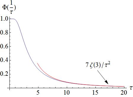
Note that

$\Pi _{++}(0,0)\rightarrow 2N_{0}{\frac {7\zeta (3)}{4\pi ^{2}T^{2}}}\Delta _{sp}^{2}$

as $\Delta _{sp}\rightarrow 0$, i.e. as $T\rightarrow T_{C}$.

That is precisely the curvature of the new minimum in the Ginzburg-Landau free energy we found before. So, at 2nd order our effective action corresponds to the action for two real free bosons, $\delta \Delta _{+}$ and $\delta \Delta _{-}$. At $q=0,i\Omega _{n}=0$, $\delta \Delta _{+}$ mode is gapped (massive), but $\delta \Delta _{-}$ mode is not gapped (massless). Physically, $\delta \Delta _{+}$ corresponds to the fluctuations of the order parameter amplitude (because we chose $\Delta _{sp}$ to be real).

Recall our discussion from many-body course:

Amplitude fluctuations are not hydrodynamic modes since they do not correspond to either conserved or to broken symmetry variable. We have to extend our approach to higher order in $\delta \Delta _{\pm }$ to describe its (rapid) decay.

$\delta \Delta _{-}$ corresponds to fluctuations along the direction of the minimum of the double well potential, where there is no barrier. It corresponds to (part of) a "phase" mode.

To determine the kinematics (of our collective modes) we need to expand $\Pi _{\mu \nu }(q,i\Omega _{n})$ in powers of Failed to parse (SVG (MathML can be enabled via browser plugin): Invalid response ("Math extension cannot connect to Restbase.") from server "https://wikimedia.org/api/rest_v1/":): {\displaystyle \vec{q}} and Failed to parse (SVG (MathML can be enabled via browser plugin): Invalid response ("Math extension cannot connect to Restbase.") from server "https://wikimedia.org/api/rest_v1/":): {\displaystyle \Omega_n} . Our small expansion parameters are

Failed to parse (SVG (MathML can be enabled via browser plugin): Invalid response ("Math extension cannot connect to Restbase.") from server "https://wikimedia.org/api/rest_v1/":): {\displaystyle \Omega_n \ll \Delta_{sp}} and Failed to parse (SVG (MathML can be enabled via browser plugin): Invalid response ("Math extension cannot connect to Restbase.") from server "https://wikimedia.org/api/rest_v1/":): {\displaystyle q \ll \frac{\Delta_{sp}}{\hbar v_F}}

(Obviously Failed to parse (SVG (MathML can be enabled via browser plugin): Invalid response ("Math extension cannot connect to Restbase.") from server "https://wikimedia.org/api/rest_v1/":): {\displaystyle q \ll k_F} )

Start with Failed to parse (SVG (MathML can be enabled via browser plugin): Invalid response ("Math extension cannot connect to Restbase.") from server "https://wikimedia.org/api/rest_v1/":): {\displaystyle \Pi_{++}}  : What we need is

Failed to parse (SVG (MathML can be enabled via browser plugin): Invalid response ("Math extension cannot connect to Restbase.") from server "https://wikimedia.org/api/rest_v1/":): {\displaystyle \Pi_{++}\left(q, i\Omega_n\right) - \Pi_{++}\left(0, 0\right)}

Failed to parse (SVG (MathML can be enabled via browser plugin): Invalid response ("Math extension cannot connect to Restbase.") from server "https://wikimedia.org/api/rest_v1/":): {\displaystyle = \frac{2}{\beta}\sum_{\omega_n}{\int{\frac{d^3k}{(2\pi)^3}\left[\frac{1}{\omega_n^2 + E_k^2} - \frac{\omega_n\left(\omega_n + \Omega_n\right) + \left(\epsilon_k - \mu\right)\left(\epsilon_{k + q} - \mu\right) - \Delta_{sp}^2}{\left(\omega_n^2 + E_k^2\right)\left(\left(\omega_n + \Omega_n\right)^2 + E_{k + q}^2\right)} - \frac{2\Delta_{sp}^2}{\left(\omega_n^2 + E_k^2\right)^2}\right]}}}

Failed to parse (SVG (MathML can be enabled via browser plugin): Invalid response ("Math extension cannot connect to Restbase.") from server "https://wikimedia.org/api/rest_v1/":): {\displaystyle = \frac{2}{\beta}\sum_{\omega_n}{\int{\frac{d^3k}{(2\pi)^3}\left[\frac{\omega_n^2 + \left(\epsilon_k - \mu\right)^2 - \Delta_{sp}^2}{\left(\omega_n^2 + E_k^2\right)^2} - \frac{\omega_n\left(\omega_n + \Omega_n\right) + \left(\epsilon_k - \mu\right)\left(\epsilon_{k + q} - \mu\right) - \Delta_{sp}^2}{\left(\omega_n^2 + E_k^2\right)\left(\left(\omega_n + \Omega_n\right)^2 + E_{k + q}^2\right)}\right]}}}

Failed to parse (SVG (MathML can be enabled via browser plugin): Invalid response ("Math extension cannot connect to Restbase.") from server "https://wikimedia.org/api/rest_v1/":): {\displaystyle = \frac{2}{\beta}\sum_{\omega_n}{\int{\frac{d^3k}{(2\pi)^3}\left[\frac{\omega_n^2 + E_k^2 - 2\Delta_{sp}^2}{\left(\omega_n^2 + E_k^2\right)^2} - \frac{\omega_n^2 + E_k^2 + \omega_n\Omega_n + \left(\epsilon_k - \mu\right)\left(\epsilon_{k + q} - \epsilon_k\right) - 2\Delta_{sp}^2}{\left(\omega_n^2 + E_k^2\right)\left(\omega_n^2 + E_k^2 + 2\omega_n\Omega_n + \Omega_n^2 + \left(\epsilon_{k + q} - \mu\right)^2 - \left(\epsilon_k - \mu\right)\right)}\right]}}}

The second term in the brackets:

Failed to parse (SVG (MathML can be enabled via browser plugin): Invalid response ("Math extension cannot connect to Restbase.") from server "https://wikimedia.org/api/rest_v1/":): {\displaystyle \frac{\omega_n^2 + E_k^2 - 2\Delta_{sp}^2 + \overbrace{\omega_n\Omega_n + \left(\epsilon_k - \mu\right)\left(\epsilon_{k + q} - \epsilon_k\right)}^{\text{small}}}{\left(\omega_n^2 + E_k^2\right)\left(\omega_n^2 + E_k^2 + \underbrace{2\omega_n\Omega_n + \Omega_n^2 + \left(\epsilon_{k + q} - \mu\right)^2 - \left(\epsilon_k - \mu\right)}_{\text{small}}\right)}}

$={\frac {\omega _{n}^{2}+E_{k}^{2}-2\Delta _{sp}^{2}+\omega _{n}\Omega _{n}+\left(\epsilon _{k}-\mu \right)\left(\epsilon _{k+q}-\epsilon _{k}\right)}{\left(\omega _{n}^{2}+E_{k}^{2}\right)^{2}}}\left[1+{\frac {2\omega _{n}\Omega _{n}+\Omega _{n}^{2}+\left(\epsilon _{k+q}-\epsilon _{k}\right)\left(\epsilon _{k+q}+\epsilon _{k}-2\mu \right)}{\omega _{n}^{2}+E_{k}^{2}}}\right]^{-1}$

Now, by Taylor expansion,

$\epsilon _{k+q}\simeq \epsilon _{k}+q\cdot \nabla \epsilon _{k}+\ldots$

and near the Fermi level we have

$q\cdot \nabla \epsilon _{k}\simeq q\cdot v_{F}$

Also note that after integrating over ${\vec {k}}$ and $\omega _{n}$, terms with odd power of $\omega _{n}$ and Failed to parse (SVG (MathML can be enabled via browser plugin): Invalid response ("Math extension cannot connect to Restbase.") from server "https://wikimedia.org/api/rest_v1/":): {\displaystyle q\cdot v_F} vanish. Keeping only terms of order Failed to parse (SVG (MathML can be enabled via browser plugin): Invalid response ("Math extension cannot connect to Restbase.") from server "https://wikimedia.org/api/rest_v1/":): {\displaystyle q^2} and Failed to parse (SVG (MathML can be enabled via browser plugin): Invalid response ("Math extension cannot connect to Restbase.") from server "https://wikimedia.org/api/rest_v1/":): {\displaystyle \Omega_n^2} we have

Failed to parse (SVG (MathML can be enabled via browser plugin): Invalid response ("Math extension cannot connect to Restbase.") from server "https://wikimedia.org/api/rest_v1/":): {\displaystyle \frac{\omega_n^2 + E_k^2 - 2\Delta_{sp}^2}{\left(\omega_n^2 + E_k^2\right)^2}\left(1 - \frac{\Omega_n^2 + \left(q\cdot v_F\right)^2}{\omega_n^2 + E_k^2}\right) - \frac{2\omega_n^2\Omega_n^2 + 2\left(\epsilon_k - \mu\right)^2\left(q\cdot v_F\right)^2}{\left(\omega_n^2 + E_k^2\right)^3} + \frac{\omega_n^2 + E_k^2 - 2\Delta_{sp}^2}{\left(\omega_n^2 + E_k^2\right)^2}\cdot\frac{4\omega_n^2\Omega_n^2 + 4\left(\epsilon_k - \mu\right)^2\left(q\cdot v_F\right)^2}{\left(\omega_n^2 + E_k^2\right)^2}}

The terms which we dropped are down by powers of Failed to parse (SVG (MathML can be enabled via browser plugin): Invalid response ("Math extension cannot connect to Restbase.") from server "https://wikimedia.org/api/rest_v1/":): {\displaystyle qk_F} and/or vanish assuming particle-hole symmetry.

Failed to parse (SVG (MathML can be enabled via browser plugin): Invalid response ("Math extension cannot connect to Restbase.") from server "https://wikimedia.org/api/rest_v1/":): {\displaystyle \Pi_{++}\left(q, i\Omega_n\right) - \Pi_{++}\left(0, 0\right)}

Failed to parse (SVG (MathML can be enabled via browser plugin): Invalid response ("Math extension cannot connect to Restbase.") from server "https://wikimedia.org/api/rest_v1/":): {\displaystyle \simeq \frac{2}{\beta}\sum_{\omega_n}{\int{\frac{d^3k}{(2\pi)^3}\frac{\omega_n^2 + E_k^2 - 2\Delta_{sp}^2}{\left(\omega_n^2 + E_k^2\right)^3}\left(\Omega_n^2 + \left(q\cdot v_F\right)^2\right)}}}

Failed to parse (SVG (MathML can be enabled via browser plugin): Invalid response ("Math extension cannot connect to Restbase.") from server "https://wikimedia.org/api/rest_v1/":): {\displaystyle + \frac{2}{\beta}\sum_{\omega_n}{\int{\frac{d^3k}{(2\pi)^3}\frac{2\omega_n^2\Omega_n^2 + 2\left(\epsilon_k - \mu\right)^2\left(q\cdot v_F\right)^2}{\left(\omega_n^2 + E_k^2\right)^3}}}}

Failed to parse (SVG (MathML can be enabled via browser plugin): Invalid response ("Math extension cannot connect to Restbase.") from server "https://wikimedia.org/api/rest_v1/":): {\displaystyle - \frac{2}{\beta}\sum_{\omega_n}{\int{\frac{d^3k}{(2\pi)^3} 4 \cdot \frac{\omega_n^2 + E_k^2 - 2\Delta_{sp}^2}{\left(\omega_n^2 + E_k^2\right)^4}\left(\omega_n^2\Omega_n^2 + \left(\epsilon_k - \mu\right)^2\left(q\cdot v_F\right)^2\right)}}}

Let's focus on Failed to parse (SVG (MathML can be enabled via browser plugin): Invalid response ("Math extension cannot connect to Restbase.") from server "https://wikimedia.org/api/rest_v1/":): {\displaystyle T = 0} . Then Failed to parse (SVG (MathML can be enabled via browser plugin): Invalid response ("Math extension cannot connect to Restbase.") from server "https://wikimedia.org/api/rest_v1/":): {\displaystyle \frac{1}{\beta}\sum_{\omega_n} \longrightarrow \int_{-\infty}^{\infty}{\frac{d\omega}{2\pi}}} Failed to parse (SVG (MathML can be enabled via browser plugin): Invalid response ("Math extension cannot connect to Restbase.") from server "https://wikimedia.org/api/rest_v1/":): {\displaystyle \Longrightarrow}

Failed to parse (SVG (MathML can be enabled via browser plugin): Invalid response ("Math extension cannot connect to Restbase.") from server "https://wikimedia.org/api/rest_v1/":): {\displaystyle \Pi_{++}\left(q, i\Omega_n\right) - \Pi_{++}\left(0, 0\right)}

Failed to parse (SVG (MathML can be enabled via browser plugin): Invalid response ("Math extension cannot connect to Restbase.") from server "https://wikimedia.org/api/rest_v1/":): {\displaystyle \simeq -2N_0\int_{-\infty}^{\infty}{\frac{d\omega}{2\pi}\int_{-\infty}^{\infty}{d\xi\frac{\omega^2 + \xi^2 - \Delta_{sp}^2}{\left(\omega^2 + \xi^2 + \Delta_{sp}^2\right)^3}\left(\Omega_n^2 + q^2\langle \left(q\cdot v_F\right)^2 \rangle_{FS}\right)}}}

Failed to parse (SVG (MathML can be enabled via browser plugin): Invalid response ("Math extension cannot connect to Restbase.") from server "https://wikimedia.org/api/rest_v1/":): {\displaystyle + 4N_0\int_{-\infty}^{\infty}{\frac{d\omega}{2\pi}\int_{-\infty}^{\infty}{d\xi\frac{\omega^2\Omega_n^2 + \xi^2q^2\langle\left(q\cdot v_F\right)^2\rangle_{FS}}{\left(\omega^2 + \xi^2 + \Delta_{sp}^2\right)^3}}}}

Failed to parse (SVG (MathML can be enabled via browser plugin): Invalid response ("Math extension cannot connect to Restbase.") from server "https://wikimedia.org/api/rest_v1/":): {\displaystyle - 8N_0\int_{-\infty}^{\infty}{\frac{d\omega}{2\pi}\int_{-\infty}^{\infty}{d\xi\frac{\omega^2 + \xi^2 - \Delta_{sp}^2}{\left(\omega^2 + \xi^2 + \Delta_{sp}^2\right)^4}\left(\omega^2\Omega_n^2 + \xi^2q^2\langle \left(q\cdot v_F\right)^2 \rangle_{FS}\right)}}}