Scaling theory of localization
localization
Before 1958, there was an old view about the behavior of an electronic system when we add a random potential. According to this view, the only effect of randomness on an electronic system is that the Bloch waves lose phase coherence on the length scale of the mean free path l, but in general the wave function stays extended throughout the sample. In 1958 Anderson proposed that the electronic systems maybe altered significantly if the disorder level is high. That means if we add a strong random potential the wave function may become localized and so the wave function decays exponentially around the random center in space,i.e., Failed to parse (SVG (MathML can be enabled via browser plugin): Invalid response ("Math extension cannot connect to Restbase.") from server "https://wikimedia.org/api/rest_v1/":): {\displaystyle \mid\psi(\overrightarrow{r})\mid\sim exp(\mid\overrightarrow{r}-\overrightarrow{r}_{0}\mid/\xi)}
where Failed to parse (SVG (MathML can be enabled via browser plugin): Invalid response ("Math extension cannot connect to Restbase.") from server "https://wikimedia.org/api/rest_v1/":): {\displaystyle \xi} is the localization length. In the strong disorder limit, and in the zero-order description we can imagine most of the eigenstates are localized around the impurity sites and then try to sum up all wave functions linearly as a perturbation to the system. This is quite confusing. What exactly do you mean here?
We could see the admixture between different orbitals will not produce an extended state because the nearby orbitals have large differences in energy and the orbitals that have the same energy are far apart in space. In both cases next order perturbation has small value and does not alter the localized states significantly.
If we ignore electron-electron and electron-phonon interactions, then in one dimension, all states are localized and it is not important how weak the disorder is. In two dimensions, they have the same behavior but in three dimensions it depends on the disorder level. That means we can have a transition between a metal and an insulator if we increase the disorder level. For weak disorder we have still extended states in the spectrum (in 3D). The dividing line between localized and extended states in the energy spectrum is called the mobility edge that is a function of energy Failed to parse (SVG (MathML can be enabled via browser plugin): Invalid response ("Math extension cannot connect to Restbase.") from server "https://wikimedia.org/api/rest_v1/":): {\displaystyle \varepsilon} and disorder strength Failed to parse (SVG (MathML can be enabled via browser plugin): Invalid response ("Math extension cannot connect to Restbase.") from server "https://wikimedia.org/api/rest_v1/":): {\displaystyle w} . This is also confusing. Mobility edge is an energy which separates localized and extended states in the pectrum. This energy is a function of disorder. But why do you say it is a function of energy?
Here we introduce the localization lenght as
Failed to parse (SVG (MathML can be enabled via browser plugin): Invalid response ("Math extension cannot connect to Restbase.") from server "https://wikimedia.org/api/rest_v1/":): {\displaystyle \xi^{-1}\equiv\underset{m\rightarrow\infty}{lim}\frac{-1}{2m}Ln\overline{\mid<0\mid G\mid m>\mid^{2}}} Please explain the meaning of m and 0 in your kets, are they position eigenstates? Why not make them vectors?
Where the bar means the average over the random potentials on each site, and G is the Green's function for system. Why we introduce the lcoalization length in this form? Assume the disorder site has energy Failed to parse (SVG (MathML can be enabled via browser plugin): Invalid response ("Math extension cannot connect to Restbase.") from server "https://wikimedia.org/api/rest_v1/":): {\displaystyle \varepsilon} and the wave function falls off exponentially as Failed to parse (SVG (MathML can be enabled via browser plugin): Invalid response ("Math extension cannot connect to Restbase.") from server "https://wikimedia.org/api/rest_v1/":): {\displaystyle exp(\frac{-m}{\xi}} ), where Failed to parse (SVG (MathML can be enabled via browser plugin): Invalid response ("Math extension cannot connect to Restbase.") from server "https://wikimedia.org/api/rest_v1/":): {\displaystyle m} is the distance from the peak. So we can calculate Green's function as below:
Failed to parse (SVG (MathML can be enabled via browser plugin): Invalid response ("Math extension cannot connect to Restbase.") from server "https://wikimedia.org/api/rest_v1/":): {\displaystyle <m\mid G(\varepsilon-i\eta)\mid0>=\sum_{n}\frac{<m\mid\varepsilon_{n}><\varepsilon_{n}\mid0>}{\varepsilon-\varepsilon_{n}-i\eta}}
Failed to parse (SVG (MathML can be enabled via browser plugin): Invalid response ("Math extension cannot connect to Restbase.") from server "https://wikimedia.org/api/rest_v1/":): {\displaystyle <m\mid G(\varepsilon-i\eta)\mid0>=V\int d\varepsilon^{'}D(\varepsilon^{'})\frac{<m\mid\varepsilon_{n}><\varepsilon_{n}\mid0>}{\varepsilon-\varepsilon_{n}-i\eta}\thickapprox\frac{V\xi}{N}D(\varepsilon)i\pi<m\mid\varepsilon>}
Where N is the number of sites in th elattice. The wave function has width Failed to parse (SVG (MathML can be enabled via browser plugin): Invalid response ("Math extension cannot connect to Restbase.") from server "https://wikimedia.org/api/rest_v1/":): {\displaystyle \xi} so a fraction Failed to parse (SVG (MathML can be enabled via browser plugin): Invalid response ("Math extension cannot connect to Restbase.") from server "https://wikimedia.org/api/rest_v1/":): {\displaystyle \frac{\xi}{N}} has overlap of order unity with site 0 ,and all the rest can be neglected. So, we have
Failed to parse (SVG (MathML can be enabled via browser plugin): Invalid response ("Math extension cannot connect to Restbase.") from server "https://wikimedia.org/api/rest_v1/":): {\displaystyle <m\mid G(\varepsilon-i\eta)\mid0>\thickapprox\frac{V\xi}{N}D(\varepsilon)i\pi e^{i\phi}e^{-\frac{m}{\xi}}}
Where Failed to parse (SVG (MathML can be enabled via browser plugin): Invalid response ("Math extension cannot connect to Restbase.") from server "https://wikimedia.org/api/rest_v1/":): {\displaystyle \phi} describes the phase of the matrix element. As you can see by using of the definition for the localization length we can get good result for Failed to parse (SVG (MathML can be enabled via browser plugin): Invalid response ("Math extension cannot connect to Restbase.") from server "https://wikimedia.org/api/rest_v1/":): {\displaystyle \xi} because we we calculate average over all random possibilities the phaseFailed to parse (SVG (MathML can be enabled via browser plugin): Invalid response ("Math extension cannot connect to Restbase.") from server "https://wikimedia.org/api/rest_v1/":): {\displaystyle (\phi)} goes to zero.
Scaling Theory of Localization
This method is the most applicable method to describe localization that was proposed by Abrahams et.al.(1979). According to this theory, there is a general behavior for materials so that if we can measure the resistance for a sample then we can predict the resistance of a sample of any other length or that sample. That means the resistance of a sample follows this relationship: Failed to parse (SVG (MathML can be enabled via browser plugin): Invalid response ("Math extension cannot connect to Restbase.") from server "https://wikimedia.org/api/rest_v1/":): {\displaystyle R(l)=R(\frac{l}{l_{0}})} where l_{0}is the length of sample that its resistance is equal to the basic quantum of resistance Failed to parse (SVG (MathML can be enabled via browser plugin): Invalid response ("Math extension cannot connect to Restbase.") from server "https://wikimedia.org/api/rest_v1/":): {\displaystyle R_{H}: R_{H}\equiv\frac{h}{e^{2}}=25.813\Omega} .
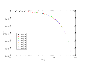
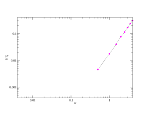
In another notation we can say there is a function for the conductance as Failed to parse (SVG (MathML can be enabled via browser plugin): Invalid response ("Math extension cannot connect to Restbase.") from server "https://wikimedia.org/api/rest_v1/":): {\displaystyle g=F(\frac{L}{\xi})} that the function F is called scaling function. In this definition the correlation length Failed to parse (SVG (MathML can be enabled via browser plugin): Invalid response ("Math extension cannot connect to Restbase.") from server "https://wikimedia.org/api/rest_v1/":): {\displaystyle (\xi} ) includes all microscopic length scales such as the Fermi wave number,mean free path etc, so this function is a single parameter scaling and these scales do not enter explicitly in the formula. We can guess the shapes of this scaling function by studying its behavior in small and large disorder. In small disorder level or very weak resistors, only occasional scattering sites cause resistivity and so in this limit they should obey the familiar macroscopic Ohm's law. That means in dimension d, Failed to parse (SVG (MathML can be enabled via browser plugin): Invalid response ("Math extension cannot connect to Restbase.") from server "https://wikimedia.org/api/rest_v1/":): {\displaystyle g\sim L^{d-2}} when R is near zero. Also in very large resistance, we expect all states to be localized and the resistivity to rise exponentially with sample length as Failed to parse (SVG (MathML can be enabled via browser plugin): Invalid response ("Math extension cannot connect to Restbase.") from server "https://wikimedia.org/api/rest_v1/":): {\displaystyle g\sim e^{-A_{d}L/L_{0}}} where Failed to parse (SVG (MathML can be enabled via browser plugin): Invalid response ("Math extension cannot connect to Restbase.") from server "https://wikimedia.org/api/rest_v1/":): {\displaystyle A_{d}} is a coefficient independent of length and only depend on dimensionality.
Abrahams proposed that instead of making guess about the shapes of g it is better to focus on the function
Failed to parse (SVG (MathML can be enabled via browser plugin): Invalid response ("Math extension cannot connect to Restbase.") from server "https://wikimedia.org/api/rest_v1/":): {\displaystyle \beta(g)\equiv\frac{dLng}{dLnL}}
So in small g, Failed to parse (SVG (MathML can be enabled via browser plugin): Invalid response ("Math extension cannot connect to Restbase.") from server "https://wikimedia.org/api/rest_v1/":): {\displaystyle \beta(g)\rightarrow} d-2 and for large g it goes to Failed to parse (SVG (MathML can be enabled via browser plugin): Invalid response ("Math extension cannot connect to Restbase.") from server "https://wikimedia.org/api/rest_v1/":): {\displaystyle Ln(\frac{g}{g_{0}})} . Here Failed to parse (SVG (MathML can be enabled via browser plugin): Invalid response ("Math extension cannot connect to Restbase.") from server "https://wikimedia.org/api/rest_v1/":): {\displaystyle g_{0}} is some constant, and also it should be noticed the dimensionless conductance g in this formula is a suitable average, such as the Thouless conductance or the typical conductance. The typical value of g is defined as Failed to parse (SVG (MathML can be enabled via browser plugin): Invalid response ("Math extension cannot connect to Restbase.") from server "https://wikimedia.org/api/rest_v1/":): {\displaystyle \rho_{typ}=exp(<log\rho(x)>)} .
Moreover, you can see the beta function is only function of g. If we assume a monotonic interpolation between these limits we can draw the schematic of the beta function.
Some important result from the behavior of the beta function:
1- In one and two dimension, the function is always negative. So in large sizes we will have no conductance or it will become very small, and we can conclude that all electronic states are localized in these dimensions. But in 2D, the situation is sensitive to our assumption on the monotonic behavior of function because if we consider the spin orbit interaction the function will become non-monotonic and we have a transition in 2D in some circumstances such as very strong the spin-orbit interaction.
2- In 3D, the beta function has zero value for a value of the conductance. This point is related to a phase transition between insulator and metal. This transition is called the Anderson transition. Also for conductance larger than a critical value, making a system larger continually decrease its resistance, and for smaller than this value it behaves inversely.
We can conclude the scaling theory makes easy to determine localization. That means rather than studying any properties of wave function or any Hamiltonian,we focus on how the solution changes with change of scale. So if we have the behavior of any sample for different scales we can say there is any localization or not. If the conductance increases with making larger it behaves like metallic phase and inversely if it decreases it behaves like insulating phase.
For example in below figure there is a transition between metals and insulators at a disorder w of around 17 because larger than this value the resistance increases with making system larger.
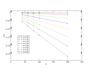
Method description and my calculations
I used transfer matrix method to calculation the conductance for one dimension, but there are some other methods like Green's function that one should use Hamiltonian to build up Green's function and then try to calculate its inverse numerically. In transfer matrix method we consider a tight binding model for a one dimension chain as
Failed to parse (SVG (MathML can be enabled via browser plugin): Invalid response ("Math extension cannot connect to Restbase.") from server "https://wikimedia.org/api/rest_v1/":): {\displaystyle H=\sum_{l}U_{l}\mid l><l\mid+t\mid l><l+1\mid+t\mid l+1><l\mid}
Where Failed to parse (SVG (MathML can be enabled via browser plugin): Invalid response ("Math extension cannot connect to Restbase.") from server "https://wikimedia.org/api/rest_v1/":): {\displaystyle U_{l}} is a random variable for a disorder system. Here we choose a uniform distribution for U between Failed to parse (SVG (MathML can be enabled via browser plugin): Invalid response ("Math extension cannot connect to Restbase.") from server "https://wikimedia.org/api/rest_v1/":): {\displaystyle -\frac{w}{2}} and Failed to parse (SVG (MathML can be enabled via browser plugin): Invalid response ("Math extension cannot connect to Restbase.") from server "https://wikimedia.org/api/rest_v1/":): {\displaystyle \frac{w}{2}} . So we have
Failed to parse (SVG (MathML can be enabled via browser plugin): Invalid response ("Math extension cannot connect to Restbase.") from server "https://wikimedia.org/api/rest_v1/":): {\displaystyle H\mid\psi>=E\mid\psi>\Rightarrow U_{l}\mid l>\psi_{l}+t\mid l>\psi_{l+1}+t\mid l+1>\psi_{l}=E\mid\psi>}
Failed to parse (SVG (MathML can be enabled via browser plugin): Invalid response ("Math extension cannot connect to Restbase.") from server "https://wikimedia.org/api/rest_v1/":): {\displaystyle U_{l}\psi_{l}+t\psi_{l+1}+t\psi_{l-1}=E\psi_{l}\Rightarrow(\begin{array}{c} \psi_{l+1}\\ \psi_{l}\end{array})=(\begin{array}{cc} \frac{E-U_{l}}{t} & -1\\ 1 & 0\end{array})(\begin{array}{c} \psi_{l}\\ \psi_{l-1}\end{array})}
Failed to parse (SVG (MathML can be enabled via browser plugin): Invalid response ("Math extension cannot connect to Restbase.") from server "https://wikimedia.org/api/rest_v1/":): {\displaystyle M=\left(\begin{array}{cc} \frac{E-U_{l}}{t} & -1\\ 1 & 0\end{array}\right)}
where M is the real-space transfer matrix. Then we can calculate total transfer matrix and calculate another transfer matrix that relate amplitudes of incident and scattered waves(T) as below:
Failed to parse (SVG (MathML can be enabled via browser plugin): Invalid response ("Math extension cannot connect to Restbase.") from server "https://wikimedia.org/api/rest_v1/":): {\displaystyle T=V^{-1}MV }
Failed to parse (SVG (MathML can be enabled via browser plugin): Invalid response ("Math extension cannot connect to Restbase.") from server "https://wikimedia.org/api/rest_v1/":): {\displaystyle V=\left(\begin{array}{cc} 1 & 1\\ \lambda^{-1} & \lambda\end{array}\right)}
Failed to parse (SVG (MathML can be enabled via browser plugin): Invalid response ("Math extension cannot connect to Restbase.") from server "https://wikimedia.org/api/rest_v1/":): {\displaystyle \lambda=\frac{1}{2}(x+\sqrt{x^{2}-4})}
where Failed to parse (SVG (MathML can be enabled via browser plugin): Invalid response ("Math extension cannot connect to Restbase.") from server "https://wikimedia.org/api/rest_v1/":): {\displaystyle x=\frac{E-U_{l}}{t}} . By taking the energy E as arbitrary parameter we can calculate T matrix and then compare it to the general matrix we can get transmission probability equal square of first element. By using of Landauer formula we can calculate conductance:
Failed to parse (SVG (MathML can be enabled via browser plugin): Invalid response ("Math extension cannot connect to Restbase.") from server "https://wikimedia.org/api/rest_v1/":): {\displaystyle g=\mid T_{p}\mid^{2}=\mid T_{11}\mid^{2}}
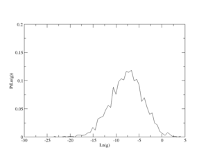
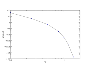
Where Failed to parse (SVG (MathML can be enabled via browser plugin): Invalid response ("Math extension cannot connect to Restbase.") from server "https://wikimedia.org/api/rest_v1/":): {\displaystyle T_{p}} is transmission probability and Failed to parse (SVG (MathML can be enabled via browser plugin): Invalid response ("Math extension cannot connect to Restbase.") from server "https://wikimedia.org/api/rest_v1/":): {\displaystyle T_{11}} is the first element of transfer matrix. It should be notice that total conductance isFailed to parse (SVG (MathML can be enabled via browser plugin): Invalid response ("Math extension cannot connect to Restbase.") from server "https://wikimedia.org/api/rest_v1/":): {\displaystyle G=\frac{2e^{2}}{h}g} and here we used typical value of conductance as g.
The Anderson transition
As we said at the transition the beta function is zero and so the conductance is independent of the system size. So by using of scaling function we conclude that the correlation length diverge at this point. Lee and Ramakrishnan in 1985 proposed this divergence behaves aswhere x is a parameter that is used to derive the system through the transition like carrier density or impurity concentration and is the critical value.
So the conductivity also has a power law dependence close to the transition for . Also for small value of the scaling function behaves as a power law . Because g is independent of L we can conclude and . This is called Wegner's scaling relation.
As you can see in 2D at the transition s=0, so the conductivity remains finite at the Anderson transition and decreases to zero discontinuously in the insulting phase.


